CSE 230: Principles of Programming Languages CSE 230

Resources - Assignments - Schedule - Grading - Policies

Summary

CSE 230 is an introduction to the Semantics of Programming Languages. Unlike most engineering artifacts, programming languages and hence, programs are mathematical objects whose properties can be formalized. The goal of CSE 230 is to to introduce you to the fundamental mental and mechanical tools required to rigorously analyze languages and programs and to expose you to recent developments in and applications of these techniques/

We shall study operational and axiomatic semantics, two different ways of precisely capturing the meaning of programs by characterizing their executions.

We will see how the lambda calculus can be used to distill essence of computation into a few powerful constructs.

We use that as a launching pad to study expressive type systems useful for for analyzing the behavior of programs at compile-time.

We will study all of the above in the context of lean, an interactive proof assistant that will help us precisely formalize and verify our intuitions about languages and their semantics.

Students will be evaluated on the basis of 4-6 programming (proving!) assignments, and a final exam.

Prerequisites

Basic functional programming e.g. as taught in UCSD CSE 130 using languages like Haskell, OCaml, Scala, Rust, and undergraduate level discrete mathematics, i.e. logic, sets, relations.

Basics

• Lecture: WLH 2005 TuTh 12:30p-1:50p
• Final Exam: 03/18/2025 Tu 11:30a-2:29p
• Podcasts: podcast.ucsd.edu
• Piazza: Piazza

Staff and Office Hours

• Ranjit Jhala: Tu, Th 2-3p (3110)
• Nico Lehmann: Th 3:30pm-5:00pm (Zoom), Fr 9:30am-11am (B240A), Zoom link in canvas
• Naomi Smith: Tu 12pm-3pm (Zoom)
• Matt Kolosick: Mo 10am-12pm (Zoom), Thursday 10am-11am (Zoom)
• Mingyao Shen: We 12-1p (B240A)
• Kyle Thompson: Mo 1-2p (B260A)

Please check the CANVAS calendar before you come in case there have been any changes.

Resources

The course is loosely based on Concrete Semantics but there is no official textbook; we will link to any relevant resources that may be needed to supplement the lecture material.

• Code from lecture

Some other useful links are:

• Lean
• Theorem Proving in Lean4
• Concrete Semantics
• Software Foundations
• Hitchhikers Guide to Logical Verification
• PL Foundations in Agda

Assignments

1. Assignment X - Github/ID due 1/17
2. Assignment 0 - Induction due 1/22

Schedule

The schedule below outlines topics, due dates, and links to assignments. The schedule of lecture topics might change slightly, but I post a general plan so you can know roughly where we are headed.

Week 1 - Basics and Induction

• Hello!
• Expressions and Types
• Datatypes and Polymorphism

Week 2 - Expressions and Evidence

• Recursion and Induction
• Handout 1-14
• Compiling Expressions to Stack Machines (Ch03)

Week 3 - Big Step Semantics

• Induction on Evidence (Ch04)
• Imperative Programs: States, Commands, Transitions
• Program Equivalence (Ch07)

Week 4 - Small Step Semantics

• Preservation and Progress (Ch09)

Week 5, 6 - Axiomatic Semantics

• Assertions, Floyd-Hoare Logic, Soundness (Ch12)
• Verification Conditions and Automatic Verification

Week 7, 8 - Simply Typed Lambda Calculus

• Terms, Types, and Typing Rules
• Denotational Semantics and Type Soundness

Week 9, 10 - Automated Verification

• Satisfiability Modulo Theories
• Flux: Refinement Type based verification for Rust

Grading

Your grade will be calculated from assignments, exam, and participation

• Participation Quizzes (15%) Most lectures will come with a 1-2 page handout, and you can submit the handout any time up until the start of the next lecture. Credit is given for reasonable effort in engaging with the material from the day on the handout.

• Programming Assignments (40%) There will be a total of 5-6 programming assigments, to be done in pairs but submitted individually.

• In Class Exams (45%) We will have three "in-class exams" Th 1/30 and Tu 2/25 and Th 3/13 each worth 15% of the grade.

Comprehensive Exam: For graduate students using this course for a comprehensive exam requirement, you must get "A" achievement on the exams.

Policies

All assignments are Closed collaboration assignments, where you cannot collaborate with others (except your partner). Of course you can ask questions on Piazza, and come to office hours etc. In particular,

• You cannot look at or use anyone else's code for the assignment
• You cannot discuss the assignment with other students
• You cannot post publicly about the assignment on the course message board (or on social media or other forums). Of course, you can still post questions about material from lecture or past assignments!

You should be familiar with the UCSD guidelines on academic integrity as well.

Late Work

You have a total of six late days that you can use throughout the quarter, but no more than four late days per assignment.

• A late day means anything between 1 second and 23 hours 59 minutes and 59 seconds past a deadline
• If you submit past the late day limit, you get 0 points for that assignment
• There is no penalty for submitting late but within the limit

Regrades

Mistakes occur in grading. Once grades are posted for an assignment, we will allow a short period for you to request a fix (announced along with grade release). If you don't make a request in the given period, the grade you were initially given is final.

Laptop/Device Policy in Lecture

There are lots of great reasons to have a laptop, tablet, or phone open during class. You might be taking notes, getting a photo of an important moment on the board, trying out a program that we're developing together, and so on. The main issue with screens and technology in the classroom isn't your own distraction (which is your responsibility to manage), it's the distraction of other students. Anyone sitting behind you cannot help but have your screen in their field of view. Having distracting content on your screen can really harm their learning experience.

With this in mind, the device policy for the course is that if you have a screen open, you either:

• Have only content onscreen that's directly related to the current lecture.
• Have unrelated content open and sit in one of the back two rows of the room to mitigate the effects on other students. I may remind you of this policy if I notice you not following it in class. Note that I really don't mind if you want to sit in the back and try to multi-task in various ways while participating in lecture (I may not recommend it, but it's your time!)

Diversity and Inclusion

We are committed to fostering a learning environment for this course that supports a diversity of thoughts, perspectives and experiences, and respects your identities (including race, ethnicity, heritage, gender, sex, class, sexuality, religion, ability, age, educational background, etc.). Our goal is to create a diverse and inclusive learning environment where all students feel comfortable and can thrive.

Our instructional staff will make a concerted effort to be welcoming and inclusive to the wide diversity of students in this course. If there is a way we can make you feel more included please let one of the course staff know, either in person, via email/discussion board, or even in a note under the door. Our learning about diverse perspectives and identities is an ongoing process, and we welcome your perspectives and input.

We also expect that you, as a student in this course, will honor and respect your classmates, abiding by the UCSD Principles of Community (https://ucsd.edu/about/principles.html). Please understand that others’ backgrounds, perspectives and experiences may be different than your own, and help us to build an environment where everyone is respected and feels comfortable.

If you experience any sort of harassment or discrimination, please contact the instructor as soon as possible. If you prefer to speak with someone outside of the course, please contact the Office of Prevention of Harassment and Discrimination: https://ophd.ucsd.edu/.

Assignments

• Assignment X - Github/ID due 1/17
• Assignment 0 - Induction due 1/22

Hello, World!

Welcome to CSE 230!

Principles of Programming Languages

i.e.

Formal Semantics

i.e.

Programs as Mathematical Objects

Computation is Specified by Programming Languages

Increased dependence implies increased need for analysis

• Safety Will this code crash?
• Security Will this code broadcast my social security number?
• Performance Will this code run in the appropriate time/space constraints?

CSE 230: PL/Programs are mathematical objects

Mental and Mechanical tools to reason about programs

Rigorous specification, analysis of PL/Programs...

... and thus, computation

CSE 230: Learning Outcomes

Goal: Mechanized Formal Semantics

Intellectual and Algorithmic tools for reasoning about program behavior

Semantics

• What does a program mean?
• What does a program do?

Formal

• We will define these objects mathematically
• We will learn how to prove things about these objects

Mechanized

• We will learn to use a precise language and tools to write these proofs

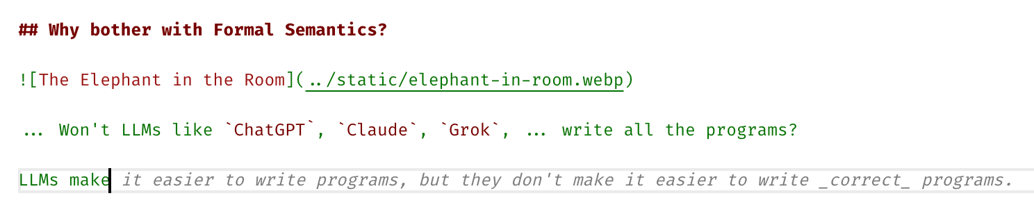
Why bother with Formal Semantics?

... Won't LLMs like ChatGPT, Claude, Grok, ... write all the programs?

Why bother with Formal Semantics?

Ranjit: What is the central thesis of "thinking fast and slow"?

Via claude -- emphasis mine.

The central thesis of "Thinking, Fast and Slow" by Daniel Kahneman is that human thinking operates in two distinct systems

• System 1 is fast, intuitive, and emotional. It operates automatically with little or no effort and no sense of voluntary control. It makes quick judgments based on familiar patterns, but is prone to systematic errors and cognitive biases.

• System 2 is slower, more deliberative, and more logical. It allocates attention to effortful mental activities that demand it, including complex calculations and careful reasoning. While more reliable than System 1, it is lazy and often defers to System 1 unless specifically engaged.

Kahneman argues that while System 1 is remarkably capable, its biases and shortcuts (heuristics) can lead to predictable errors in judgment. Many of our decision-making problems stem from System 1 making quick judgments when slower, more analytical System 2 thinking would be more appropriate. Yet we can't simply turn off System 1 - both systems serve important functions and work together to shape our thoughts and decisions.

System 1 == LLMs vs System 2 == Formal Semantics

( H/T to Adithya Murali for the analogy... )

Why Formal Semantics in the age of LLMs?

LLMs ==> more code ==> more bugs

1. More need to really understand code!

2. More tools to help understand code!

(i.e. The more you rely on "system 1", the more you need "system 2"!)

Medium of instruction: Lean

Lean is a programming language and theorem prover

• Used to write mathematical proofs that are automatically verified by the computer

• Similar to many other theorem provers like Rocq (Coq), Agda, Isabelle, etc.

• Used in academia and industry for formal verification

Two main features for CSE 230

• Helps define and prove things about languages and programs

• Example of state-of-the-art programming language

A quick taste of lean...

You can define functions...

def sum (n: Nat) : Nat :=
  match n with
  | 0 => 0                  -- if n is 0, return 0
  | m + 1 => m + 1 + sum m  -- if n is m+1, return (m+1) + sum m

sum 5 ==> 5 + sum 4 ==> 5 + 4 + sum 3 ==> 5 + 4 + 3 + 2 + 1 + sum 0 ==> 5 + 4 + 3 + 2 + 1 + 0

You can evaluate i.e. "run" them ...

#eval sum 100

You can automatically check simple facts about them...

def i_had_soup_for_lunch : sum 100 = 5050 :=
  rfl

And finally, you can write proofs for more complicated facts ...

theorem sum_eq : ∀ (n: Nat),  2 * sum n = n * (n + 1) := by
  intro n
  induction n
  . case zero =>
    rfl
  . case succ =>
    rename_i m ih
    simp_arith [sum, ih, Nat.mul_add, Nat.mul_comm]

Logistics

Lets talk about the course logistics...

Course Outline

About 2-ish weeks per topic, roughly following Concrete Semantics by Tobias Nipkow and Gerwin Klein

Part I: Basics of Lean and Proofs

• Expressions & Types
• Datatypes & Proofs
• Recursion & Induction & Evidence

Part II: Operational Semantics

• Big Step Semantics
• Small Step Semantics

Part III: Axiomatic Semantics

• Floyd-Hoare Logic
• VC Generation and Automated Verification

Part IV: Types

• Simply Typed Lambda Calculus
• Denotational Type Soundness

Prerequisites

Basic functional programming

• e.g. as taught in UCSD CSE 130
• using languages like Scheme, Haskell, Ocaml, Scala, Rust, ...

Undergraduate level discrete mathematics,

• e.g. as taught in UCSD CSE 20
• boolean logic, quantifiers, sets, relations, ...

You may be able to take 130 if you're unfamiliar with the above but ...

Grading

Your grade will be calculated from assignments, exam, and participation

• Handouts (15%) Most lectures will come with a 1-2 page handout, and you can submit the handout any time up until the start of the next lecture. Credit is given for reasonable effort in engaging with the material from the day on the handout.

• Programming Assignments (40%) There will be a total of 5-6 programming assigments, to be done in pairs but submitted individually.

• In Class Exams (45%) We will have three "in-class exams" Th 1/30 and Tu 2/25 and Th 3/13 each worth 15% of the grade.

Comprehensive Exam: For graduate students using this course for a comprehensive exam requirement, you must get "A" achievement on the exams.

Assignments (5-6)

• You can work with a partner, but submit individually
• Github Classroom + Codespaces

Assignment 0 Fill out this form to link UCSD ID and Github

And now, let the games begin...!

Expressions, Types and Functions

This material is based on sections 1-3 of Functional Programming in Lean

Expressions

In lean, programs are built from expressions which (if well-typed) have a value.

Lean expressions are mathematical expressions as in Haskell, Ocaml, etc.

• variables get a "bound" to a single value (no "re-assignment"),
• expressions always evaluate to the same value ("no side effects")
• if two expressions have the same value, then replacing one with the other will not cause the program to compute a different result.

To evaluate an expression, write #eval before it in your editor, and see the result by hovering over #eval.

#eval 1 + 2

#eval 3 * 4

#check 1 + 2 * 3 + 4

Types

Every lean expression has a type.

The type tells lean -- without evaluating the expression -- what kind of value it will produce.

Why do Programming Languages need types???

Lean has a very sophisticated type system that we will learn more about soon...

To see the type of an expression, write #check before it in your editor,

Primitive: Nat

Lean has a "primitive" type Nat for natural numbers (0, 1, 2, ...) that we saw in the expressions above.

#check 1      -- Nat (natural number i.e. 0, 1, 2,...)

#check 1 + 2  -- Nat

QUIZ What is the value of the following expression?

#eval (5 - 10 : Int)


/-

(A) 5                 0%
(B) 10                0%
(C) -5                30%
(D) 0                 5%
(E) None of the above 17%

-/

Type Annotations

Sometimes lean can infer the type automatically.

But sometimes we have to (or want to) give it an annotation.

Primitive: Int

#check (1 : Int)      -- Int (..., -2, -1, 0, 1, 2,...)

#check (1 + 2 : Int)  -- Int

QUIZ What is the value of the following expression?

#eval (5 - 10 : Int)

Primitive: Float

#check 1.1      -- Float

#eval 1.1 + 2.2

Primitive: Bool

#eval true
#check true   -- Bool

#eval false
#check false  -- Bool

#eval true  && true
#eval true  && false
#eval false && true
#eval false && false

#eval true  || true
#eval true  || false
#eval false || true
#eval false || false

-- #eval false + 10    -- type error!

Primitive: String

#eval "Hello, " ++ "world!"
#check "Hello, " ++ "world!"  -- String

-- #eval "Hello, " ++ 10   -- type error!

-- #eval "Hello, " ++ world   -- unknown identifier!

Definitions

We can name expressions using the def keyword.

def hello := "hello"
def world := "world"
def one := 1
def two := 2
def five_plus_ten   := 5 + 10
def five_minus_ten  := 5 - 10
def five_minus_ten' : Int := 5 - 10

You can now #check or #eval these definitions.

#check hello
#eval hello
#eval hello ++ world
#eval five_minus_ten
#eval five_minus_ten'

Functions

In lean, functions are also expressions, as in the λ-calculus.

#check (fun (n : Nat) => n + 1)         -- Nat -> Nat
#check (λ (n : Nat) => n + 1)           -- Nat -> Nat

#check (fun (x y : Nat) => x + y)       -- Nat -> (Nat -> Nat)
#check (λ (x y : Nat) => x + y)         -- Nat -> Nat -> Nat
#check (λ (x : Nat) => λ (y: Nat) => x + y)         -- Nat -> Nat -> Nat

QUIZ What is the type of the following expression?

Nat -> Nat -> Bool

#check (fun (x y : Nat) => x > y)

Function Calls

You can call a function by putting the arguments in front

#eval (fun x => x + 1) 10

#eval ((fun x y => x + y) 100) 200

/-
((fun x y => x + y) 100) 200
==
((λ x => (λ y => x + y)) 100) 200
==
(( (λ y => 100 + y))) 200
==
100 + 200
==
300
-/

QUIZ What is the value of the following expression?

#eval (fun x y => x > y) 10 20

Function Definitions

Of course, it is more convenient to name functions as well, using def since naming allows us to reuse the function in many places.

def inc := fun (x : Int)  => x + 1

def inc'(x: Int) := x + 1

#eval inc 10
#eval inc 20
-- #eval inc true  -- type error!

def add := fun (x y : Nat) => x + y
def add' (x y : Nat) := x + y

#eval add 10 20
#eval add' 10 20

It is often convenient to write the parameters of the function to the left

The below definitions of inc' and add' are equivalent to the above definitions of inc and add.

def inc'' (x : Int) : Int := x + 1

#eval inc'' 10     -- 11


def add'' (x y : Nat) : Nat := x + y

#eval add'' 10 20  -- 30

EXERCISE Write a function max that takes two Nats and returns the maximum of the two.

EXERCISE Write a function max3 that takes three Nats and uses max to compute the maximum of all three

EXERCISE Write a function joinStringsWith of type String -> String -> String -> String that creates a new string by placing its first argument between its second and third arguments.

def mymax (x y : Nat) := if x > y then x else y

def mymax3 (x y z : Nat) := mymax x (mymax y z)

#eval mymax 67 92

-- #eval joinStringsWith ", " "this" "that"  -- "this, that"
-- #check joinStringsWith ", " -- **QUIZ** What is the type of the expression on the left?

EXERCISE Write a function volume of type Nat -> Nat -> Nat -> Nat which computes the volume of a brick given height, width, and depth.

Datatypes and Recursion

This material is based on sections 5,6 of Functional Programming in Lean

Datatypes

So far, we saw some "primitive" or "built-in" types like Nat, Bool etc.

The "primitive" Bool type is actually defined as a datatype in the standard library:

The type has two constructors

• Bool.false
• Bool.true.

Which you can think of as "enum"-like constructors.

Like all (decent) modern languages, Lean lets you construct new kinds of datatypes. Let's redefine Bool locally, just to see how it's done.

namespace MyBool

inductive Bool : Type where
  | false : Bool
  | true  : Bool
  deriving Repr

#eval Bool.true

Pattern Matching

The constructors let us produce or build values of the datatype.

The only way to get a Bool is by using the Bool.true or Bool.false constructors.

In contrast, pattern-matching lets us consume or use the values of that datatype...

Lets write a function neg that takes a Bool and returns the opposite Bool, that is

• when given Bool.true, neg should return Bool.false
• when given Bool.false, neg should return Bool.true

def neg (b: Bool) :=
  match b with
  | Bool.true  => Bool.false
  | Bool.false => Bool.true

Lets test it to make sure the right thing is happening

#eval neg Bool.true
#eval neg Bool.false

Our first "theorem" ... let us prove that neg true is false by

1. defining a variable neg_true_eq_false (you can call it whatever you like...)
2. whose type is the proposition neg Bool.true = Bool.false we want to "prove"
3. whose body is the proof of the proposition.

For now, lets just write by sorry for the "proof".

def neg_b_neq : ∀ (b:Bool), ¬ (neg b = b) := by
  intros b
  cases b <;> simp [neg]

def neg_neg_b_eq : ∀ (b:Bool), neg (neg b) = b := by
  intros b
  cases b <;> simp [neg]

def neg_true_eq_false : neg Bool.true = Bool.false := by
  rfl

foo <;> bar

Goals

How shall we write the proof?

Well, you can see the goal by

1. putting the cursor next to the by (before sorry)
2. looking at the Lean Infoview on the right in vscode

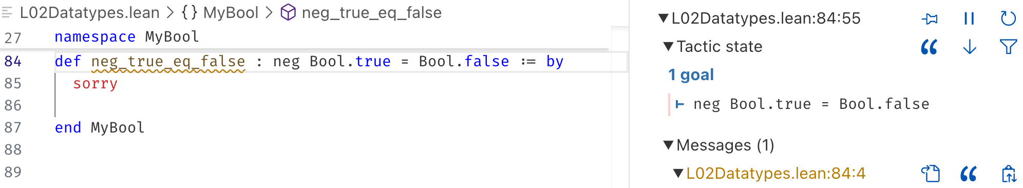
A goal always looks like h1, h2, h3, ... ⊢ g where

• h1, h2, h3 etc. are hypotheses i.e. what we have, and
• <g> is the goal i.e. what we want to prove.

In this case, the hypotheses are empty and the goal is neg Bool.true = Bool.false.

Tactics

Proofs can be difficult to write (in this case, not so much).

Fortunately, lean will help us build up the proof by

• giving us the goal that
• we can gradually simplify, split ...
• till we get simple enough sub-goals that it can solve automatically.

TACTIC rfl: The most basic tactic is rfl which abbreviates reflexivity, which is a fancy way of saying "evaluate the lhs and rhs and check if they are equal".

EXERCISE: Write down and "prove" the theorem that neg false is true.

EXERCISE What other "facts" can you think up (and prove!) about neg?

Next, lets try to prove a fact about how neg behaves on all Bool values. For example, lets try to prove that when we neg a Bool value b two times we get back b.

def neg_neg : ∀ (b: Bool), neg (neg b) = b := by
  sorry

This time we cannot just use rfl -- try it and see what happens!

In its own way, lean is saying "I can't tell you (evaluate) what neg b is because I don't know what b is!"

TACTIC intros: First, we want to use the intros tactic which will "move" the ∀ (b: Bool) from the goal into a plain b : Bool hypothesis. That is, the intros tactic will change the goal from ∀ (b: Bool), neg (neg b) = b to b : Bool ⊢ neg (neg b) = b, meaning that our task is now to prove that neg (neg b) = b assuming that b is some Bool valued thing.

Of course, we still cannot use rfl because lean does not know what neg b until b itself has some concrete value.

TACTIC cases: The path forward in this case is to use the cases tactic which does a case analysis on b, i.e. tells lean to split cases on each of the possible values of b --- when it is true and when it is false. Now, when you put your cursor next to cases b you see the two subgoals

• case false which is ⊢ neg (neg Bool.false) = Bool.false
• case true which is ⊢ neg (neg Bool.true) = Bool.true

Each case (subgoal) can be proved by rfl so you can complete the proof as

def neg_neg_1 : ∀ (b : Bool), neg (neg b) = b := by
  intros b
  cases b
  rfl
  rfl

However, I prefer to make the different subgoals more "explicit" by writing

def neg_neg_2 : ∀ (b : Bool), neg (neg b) = b := by
  intros b
  cases b
  . case false => rfl
  . case true => rfl

Conjunction Lets write an and function that

• takes two Bools and
• returns a Bool that is true if both are true and false otherwise.

def and (b1 b2: Bool) : Bool :=
  match b1, b2 with
  | Bool.true, Bool.true => Bool.true
  | _        , _         => Bool.false

and is Commutative Lets try to prove that and is commutative, i.e. and b1 b2 = and b2 b1. You can start off with intros and then use cases as before, but we may have to do case analysis on both the inputs!

theorem and_comm : ∀ (b1 b2 : Bool), and b1 b2 = and b2 b1 := by
  sorry

TACTIC COMBINATOR <;>: It is a bit tedious to repeat the same sub-proof so many times! The foo <;> bar tactic combinator lets you chain tactics together so by first applying foo and then applying bar to each sub-goal generated by foo. We can use <;> to considerably simplify the proof. In the proof below, move your mouse over the cases b1 <;> cases b2 <;> ... line and see how the goals change in the Lean Infoview panel.

theorem and_comm' : ∀ (b1 b2 : Bool), and b1 b2 = and b2 b1 := by
  -- use the <;> tactic combinator
  sorry

Disjunction Lets write an or function that

• takes two Bools and
• returns a Bool that is true if either is true and false otherwise.

def or (b1 b2: Bool) : Bool := sorry

EXERCISE Complete the proof of the theorem that or is commutative, i.e. or produces the same result no matter the order of the arguments.

theorem or_comm : ∀ (b1 b2 : Bool), or b1 b2 = or b2 b1 := by
  sorry

end MyBool

Recursion

Bool is a rather simple type that has just two elements --- true and false.

Pretty much all proofs about Bool can be done by splitting cases on the relevant Bool values and then running rfl (i.e. via a giant "case analysis").

Next, lets look at a more interesting type, which has an infinite number of values.

namespace MyNat

inductive Nat where
  | zero : Nat
  | succ : Nat -> Nat
  deriving Repr

open Nat

Zero, One, Two, Three, ... infinity

Unlike Bool there are infinitely many Nat values.

def n0 : Nat :=                  zero
def n1 : Nat :=             succ zero
def n2 : Nat :=       succ (succ zero)
def n3 : Nat := succ (succ (succ zero))

This has two related consequences.

First, we cannot write interesting functions over Nat just by brute-force enumerating the inputs and outputs as we did with and and or; instead we will have to use recursion.

Second, we cannot write interesting proofs over Nat just by brute-force case-splitting over the values as we did with and_comm and or_comm; instead we will have to use induction.

Addition

Lets write a function to add two Nat values.

def add (n m: Nat) : Nat :=
  match n with
  | zero => m
  | succ n' => succ (add n' m)

example : add n1 n2 = n3 := by rfl

Adding Zero

Next, lets try to prove some simple facts about add for example

theorem add_zero_left : ∀ (n: Nat), add zero n = n := by
  intros
  rfl

The proof of add_zero_left is super easy because it is literally (part of) the definition of add which tells lean that it obeys two equations

add zero      m = m
add (succ n') m = succ (add n' m)

So the rfl applies the first equation and boom we're done.

Adding Zero on the Right

However, lets see what happens if we flip the order of the arguments, so that the second argument is zero

theorem add_zero' : ∀ (n: Nat), add n zero = n := by
  intros n
  sorry

Boo! Now the proof fails because the equation does not apply!

"Calculation" or "Equational Reasoning"

In fact, lets us try to see why the theorem is even true, slowly working our way up the Nat numbers.

  add zero  zero
    { by def of add }
    ===> zero                     ... (0)

  add (succ zero) zero
    { by def of add }
    ===> succ (add zero zero)
    { by (0) }
    ===> succ zero                ... (1)

  add (succ (succ (zero))) zero
    { by def }
    ===> succ (add (succ zero) zero)
    { by (1) }
    ===> succ (succ zero)         ... (2)

  add (succ (succ (succ (zero)))) zero
    { by def }
    ===> succ (add (succ (succ zero)) zero)
    { by (2) }
    ===> succ (succ (succ zero))  ... (3)

calc mode

lean has a neat calc mode that lets us write the above proofs (except, they are actually checked!)

theorem add_0 : add zero zero = zero := by
  calc
    add zero zero = zero := by simp [add] -- just apply the

theorem add_1 : add (succ zero) zero = succ zero := by
  calc
    add (succ zero) zero
      = succ (add zero zero) := by simp [add]
    _ = succ zero            := by simp [add_0]

theorem add_2 : add (succ (succ zero)) zero = succ (succ zero) := by
  calc
    add (succ (succ zero)) zero
      = succ (add (succ zero) zero) := by simp [add]
    _ = succ (succ zero)            := by simp [add_1]

theorem add_3 : add (succ (succ (succ zero))) zero = succ (succ (succ zero)) := by
  calc
    add (succ (succ (succ zero))) zero
      = succ (add (succ (succ zero)) zero) := by simp [add]
    _ = succ (succ (succ zero))            := by simp [add_2]

Proof by Induction

Notice that each of the proofs above is basically the same:

To prove the fact add_{n+1} we

1. apply the definition of add and then
2. recursively use the fact add_{n}!

Recursion

Lets us define add for each Nat by reusing the definitions on smaller numbers

Induction

Lets us prove add_n for each Nat by reusing the proofs on smaller numbers

theorem add_zero : ∀ (n: Nat), add n zero = n := by
  intros n
  induction n
  . case zero       => simp [add]
  . case succ n' ih => simp [add, ih]

end MyNat

Polymorphism

lean also lets you define polymorphic types and functions.

For example, here is the definition of a List type that can hold any kind of value

namespace MyList

inductive List (α : Type) where
  | nil : List α
  | cons : α -> List α -> List α
  deriving Repr

open List

List constructors

Just like Nat has a

• "base-case" constructor (zero) and
• "inductive-case" constructor (succ)

A List α also has two constructors:

• "base-case" constructor (nil) and
• "inductive-case" constructor (cons)

NOTE: You can type the α by typing a \ + a

So we can create different types of lists, e.g.

def list0123 : List Int := cons 0 (cons 1 (cons 2 (cons 3 nil)))
def list3210 : List Int := cons 3 (cons 2 (cons 1 (cons 0 nil)))
def listtftf : List Bool := cons true (cons false (cons true (cons false nil)))

Appending Lists

Lets write a small function to append or concatenate two lists

To do so, we match on the cases of the first list xs

• If xs is nil then the result is just the second list
• If xs is of the form cons x xs' then we recursively app xs' ys and cons x in front

def app {α : Type} (xs ys: List α) : List α :=
  match xs with
  | nil => ys
  | cons x xs' => cons x (app xs' ys)

Just like with add the above definition tells lean that app satisfies two equations

1. ∀ ys, app nil ys = ys
2. ∀ x xs' ys, app (cons x xs') ys = cons x (app xs' ys)

example : app                 nil   (cons 2 (cons 3 nil)) =                 cons 2 (cons 3 nil)   := by rfl
example : app         (cons 1 nil)  (cons 2 (cons 3 nil)) =         cons 1 (cons 2 (cons 3 nil))  := by rfl
example : app (cons 0 (cons 1 nil)) (cons 2 (cons 3 nil)) = cons 0 (cons 1 (cons 2 (cons 3 nil))) := by rfl

Digression: Implicit vs Explicit Parameters

The α -- representing the Type of the list elements -- is itself a parameter for the app function.

• The {..} tells lean that it is an implicit parameter vs
• The (..) we usually use for explicit parameters

An implicit parameter, written {...} is a parameter that lean tries to automatically infer at call-sites, based on the context, for example

def add (n : Nat) (m : Nat) : Nat := n + m
#eval add 3 4  -- Must provide both arguments: 7

An explicit parameter, written (...) is the usual kind where you have to provide at call-sites, for example

def singleton {α : Type} (x: α) : List α := cons x nil
#eval singleton 3

Induction on Lists

app is sort of like add but for lists. For example, it is straightforward to prove "by definition" that

theorem app_nil_left: ∀ {α : Type} (xs: List α), app nil xs = xs := by
  intros
  rfl

However, just like add_zero we need to use induction to prove that

theorem app_nil : ∀ {α : Type} (xs: List α), app xs nil = xs := by
  sorry

Because in the cons x xs' case, we require the fact that app_nil holds for the smaller tail xs', i.e that app xs' nil = xs', which the induction tactic will give us as the hypothesis that we can use.

Associativity of Lists

theorem app_assoc : ∀ {α : Type} (xs ys zs: List α), app (app xs ys) zs = app xs (app ys zs) := by
  sorry

end MyList

set_option pp.fieldNotation false

Datatypes and Recursion

This material is based on

• Chapter 2 of Concrete Semantics
• Induction Exercises by James Wilcox

namespace MyNat

inductive Nat where
  | zero : Nat
  | succ : Nat -> Nat
  deriving Repr

open Nat

def add (n m : Nat) : Nat :=
  match n with
  | zero => m
  | succ n' => succ (add n' m)

Trick 1: Helper Lemmas

Example add_comm

Let's try to prove that add is commutative; that is, that the order of arguments does not matter.

If we plunge into trying a direct proof-by-induction, we get stuck at two places.

1. What is the value of add m zero ?
2. What is the value of add m (succ n) ?

It will be convenient to have helper lemmas that tell us that

1. ∀ m, add m zero = m
2. ∀ n m, add n (succ m) = succ (add n m)

theorem add_comm : ∀ (n m: Nat), add n m = add m n := by
  intros n m
  induction n
  sorry

end MyNat

open List

Example rev_rev

Lets look at another example where we will need helper lemmas.

Appending lists

def app {α : Type} (xs ys: List α) : List α :=
  match xs with
  | [] => ys
  | x::xs' => x :: app xs' ys

/-
app [] [3,4,5] = [3,4,5]

app (2::[]) [3,4,5] = [3,4,5]
==>
2 :: [3,4,5]
==>
[2,3,4,5]
-/

example : app [] [3,4,5] = [3,4,5] := rfl
example : app [0,1,2] [3,4,5] = [0,1,2,3,4,5] := rfl

Reversing lists

def rev {α : Type} (xs: List α) : List α :=
 match xs with
  | [] => []
  | x :: xs' => app (rev xs') [x]

example : rev [] = ([] : List Int) := rfl
example : rev [3] = [3] := rfl
example : rev [2,3] = [3,2] := rfl
example : rev [0,1,2,3] = [3,2,1,0] := rfl
example : rev (rev [0,1,2,3]) = [0,1,2,3] := rfl

rev [0,1,2,3] => rev (0 :: [1,2,3]) => app (rev [1,2,3]) [0] => app [3,2,1] [0] => [3,2,1,0]

Now, lets prove that the above was not a fluke: if you reverse a list twice then you get back the original list.

theorem rev_app : ∀ {α : Type} (xs ys : List α),
  rev (app xs ys) = app (rev ys) (rev xs) := by
    sorry

/-
rev (app xs ys) == app (rev ys) (rev xs)
rev (app [x1,x2,x3,...xn] [y1...ym])
== rev [x1...xn, y1...ym]
== [ym ... y1, xn ... x1]
== app [ym ... y1] [xn ... x1]
== app (rev ys) (rev xs)

-- |- rev (app (rev xs') [x]) = x :: xs'
      ==>
      app (rev [x]) (rev (rev xs'))
-/

theorem rev_rev : ∀ {α : Type} (xs: List α), rev (rev xs) = xs := by
  intros α xs
  induction xs
  . case nil =>
    rfl
  . case cons x xs' ih =>
    simp [rev, rev_app, app, ih]

Yikes. We're stuck again. What helper lemmas could we need?

Trick 2: Generalizing the Variables

Consider the below variant of add.

How is it different than the original?

open MyNat.Nat

def itadd (n m: MyNat.Nat) : MyNat.Nat :=
  match n with
  | zero => m
  | succ n' => itadd n' (succ m)

/-
  itadd (s s s z) (s s s s s z)
  =>
  itadd (s s z) (s s s s s s z)
  =>
  itadd (s z) (s s s s s s s z)
  =>
  itadd (z) (s s s s s s s s z)
  =>
  (s s s s s s s s z)
-/


example : itadd (succ (succ zero)) (succ zero) = succ (succ (succ zero)):= by rfl

Lets try to prove that itadd is equivalent to add.

add n' (succ m) == succ (add n' m)

theorem add_succ : ∀ (n m), MyNat.add n (succ m) = succ (MyNat.add n m) := by
 sorry

theorem itadd_eq : ∀ (n m), itadd n m = MyNat.add n m := by
  intros n
  induction n
  . case zero => simp [itadd, MyNat.add]
  . case succ n' ih =>
    simp [MyNat.add, itadd, add_succ, ih]

Ugh! Why does the proof fail???

We are left with the goal

m n' : MyNat.Nat
ih : itadd n' m = MyNat.add n' m
⊢ itadd n' (succ m) = succ (MyNat.add n' m)

IH is too weak

In the goal above, the ih only talks about itadd n m but says nothing about itadd n (succ m). In fact, the IH should be true for all values of m as we do not really care about m in this theorem. That is, we want to tell lean that the ih should be

m n' : MyNat.Nat
ih : ∀ m, itadd n' m = MyNat.add n' m
⊢ itadd n' (succ m) = succ (MyNat.add n' m)

Generalizing We can do so, by using the induction n generalizing m which tells lean that

• we are doing induction on n and
• we don't care about the value of m

Now, go and see what the ih looks like in the case succ ...

This time we can actually use the ih and so the proof works.

theorem add_succ : ∀ (n m), MyNat.add n (succ m) = succ (MyNat.add n m) := by
 sorry

theorem itadd_eq' : ∀ (n m: MyNat.Nat), itadd n m = MyNat.add n m := by
  intros n m
  induction n generalizing m
  case zero => simp [MyNat.add, itadd]
  case succ => simp [MyNat.add, MyNat.add_succ, itadd, *]

Trick 3: Generalizing the Induction Hypothesis

Often, the thing you want to prove is not "inductive" by itself. Meaning, that you want to prove a goal ∀n. P(n) but in fact you need to prove something stronger like ∀n. P(n) /\ Q(n) or even ∀n m, Q(n, m) which then implies your goal.

Example: Tail-Recursive sum

sum 3
=>
3 + sum 2
=>
3 + 2 + sum 1
=>
3 + 2 + 1 + sum 0
=>
3 + 2 + 1 + 0

def sum (n : Nat) : Nat :=
  match n with
  | 0 => 0
  | n' + 1 => n + sum n'

def loop (n res : Nat) : Nat :=
  match n with
  | 0      => res
  | n' + 1 => loop n' (res + n)

def sum_tr (n: Nat) := loop n 0

-- loop (n' + 1) 0 == sum (n' + 1)
-- loop a 0  == sum a
-- loop n res  == (sum n) + res

theorem loop_sum : ∀ n res, loop n res = (sum n) + res := by
  intros n res
  induction n generalizing res
  . case zero =>
    simp [loop, sum]
  . case succ n' ih =>
    simp_arith [loop, sum, ih]

theorem sum_eq_sum_tr : ∀ n, sum_tr n = sum n := by
  simp [sum_tr, loop_sum]




/-

fn sum(mut n: Nat) -> Nat {
  let mut res = 0
  while let S n' = n {
    res = res + n;
    n   = n';
  }
  res
}
-/

Tail-Recursively Summing

In an iterative language you might write a loop to sum the numbers n + n-1 + ... + 0 e.g.

#![allow(unused)]
fn main() {
fn sum_tr(mut n: Nat) {
  let mut acc = 0;
  while let succ m = n {
    acc += n;
    n = m
  }
  return acc
}
}

We can write the above with tail-recursion

• The recursive call is the "last thing" the function does
• That is, the recursive result is returned without any further computation

NOTE: Go and look at itadd; is it tail recursive?

-- def sum_tr (n acc : Nat) : Nat :=
--   match n with
--   | 0 => acc
--   | n' + 1 => sum_tr n' (n + acc)

-- def sum' (n: Nat) := sum_tr n 0

Lets try to prove that sum and sum' always compute the same result.

theorem sum_eq_sum' : ∀ n, sum n = sum' n := by
  intros n
  induction n
  sorry

Oops, we are stuck.

We need to know something about sum_tr n' (n' + 1) but what?

Can you think of a suitable helper lemma, which would let us directly prove sum_eq_sum'?

theorem helper: ∀ n acc, sum_tr n acc = sum n + acc := by ...

theorem sum_eq_sum' : ∀ n, sum' n = sum n := by
  intros
  simp_arith [sum', helper]

open List

Example: Tail-Recursive sum_list

Summing a List*

def sum_list (xs : List Nat) : Nat :=
  match xs with
  | [] => 0
  | x ::xs' => x + sum_list xs'

Tail-Recursively Summing a List*

In an iterative language you might write a loop to sum the elements of a list, e.g.

#![allow(unused)]
fn main() {
fn sum_list(xs: List<Nat>) {
  let mut acc = 0;
  while let cons x ys = xs {
    acc += x;
    xs = ys
  }
  return acc
}
}

We can write the above with tail-recursion (where the recursive call is the "last thing") that the function does. (Hint: Go and look at itadd; is it tail recursive?)

def sum_list_tr (xs : List Nat) (acc : Nat): Nat :=
  match xs with
  | [] => acc
  | x :: ys => sum_list_tr ys (acc + x)

def sum_list' (xs: List Nat) := sum_list_tr xs 0

Can you figure out a suitable helper lemma that would let us complete the proof of sum_list_eq_sum_list' below?

theorem sum_list'_eq : ∀ (xs acc), sum_list_tr xs acc = sum_list xs + acc := by
  sorry

theorem sum_list_eq_sum_list' : ∀ xs, sum_list' xs = sum_list xs := by
  intros xs
  simp_arith [sum_list', sum_list'_eq]

Example: Tail-Recursive Reverse

rev_tr [0,1,2,3]
=>
loop [0,1,2,3] []
=>
loop [1,2,3] [0]
=>
loop [2,3] [1, 0]
=>
loop [3] [2, 1, 0]
=>
loop [] [3, 2, 1, 0]
=>
[3,2,1,0]

def rev_tr {α : Type} (xs res: List α) : List α :=
  match xs with
  | [] => res
  | x ::xs' => rev_tr xs' (x :: res)

def rev' (xs: List α) := rev_tr xs []

example : rev' [0,1,2,3] = [3,2,1,0] := by rfl

Can you figure out a suitable helper lemma rev_tr_app that would let us complete the proof of rev_eq_rev' below?

rev_tr xs [] == rev xs

rev_tr xs res
  == [xn, ...x3, x2,x1, 99]
  == rev xs ++ res

theorem app_nil : ∀ {α : Type} (xs: List α), app xs [] = xs := by
  sorry

theorem rev_tr_helper_theorem : ∀ {α : Type} (xs res : List α),
  rev_tr xs res = app (rev xs) res := by sorry

theorem rev_eq_rev' : ∀ {α : Type} (xs: List α), rev' xs = rev xs := by
  intros α xs
  simp [rev', rev_tr_helper_theorem, app_nil]

Example: Tail-Recursive Evaluator

Arithmetic Expressions

inductive Aexp : Type where
  | const : Nat -> Aexp
  | plus  : Aexp -> Aexp -> Aexp
  deriving Repr

open Aexp

def two_plus_three := plus (const 2) (const 3)

     alice_plus
    /          \
   bob_const   bob_const
   |            |
   2            3

Evaluating Expressions

def eval (e: Aexp) : Nat :=
  match e with
  | const n => n
  | plus e1 e2 => eval e1 + eval e2

#eval eval two_plus_three

def eval_acc (e: Aexp) (res: Nat) : Nat :=
  match e with
  | const n => n + res
  | plus e1 e2 => eval_acc e2 (eval_acc e1 res)

def eval' (e: Aexp) := eval_acc e 0

example : eval' two_plus_three = eval two_plus_three := by rfl

eval' two_plus_three
=>
eval' (plus (const 2) (const 3))
=>
eval_acc (plus (const 2) (const 3)) 0
=>
eval_acc (const 3) (eval_acc (const 2) 0)
=>
eval_acc (const 3) ( 2 + 0)
=>
eval_acc (const 3) 2
=>
3 + 2
=>
5

QUIZ: Is eval_acc tail recursive?

Lets try to prove that eval' and eval are "equivalent".

Can you figure out a suitable helper lemma that would let us complete the proof of eval_eq_eval'?

theorem magic_theorem : ∀ e res, eval_acc e res = eval e + res := by
  intros e res
  induction e generalizing res
  . case const n => rfl
  . case plus e1 e2 ih1 ih2 =>
    simp_arith [eval, eval_acc, ih1, ih2]

theorem eval_eq_eval' : ∀ e, eval e = eval' e := by
  intros e
  simp [eval', magic_theorem]

Trick 4: Functional Induction

Based on Joachim Breitner's notes on Functional Induction

def len (xs: List α) : Nat :=
  match xs with
  | [] => 0
  | _::xs' => 1 + len xs'

def alt (xs ys : List α) : List α :=
  match xs, ys with
  | [], ys => ys
  | xs, [] => xs
  | x::xs', y::ys' => x :: y :: alt xs' ys'

#eval alt [1,2,3,4] [10]

First, lets try a "brute force" proof.

exp ::= const c | var | plus exp exp | mult exp exp

(plus
  (mult
    (const 7)
    (mult (var (mult var var)))))
  (plus
    (mult (const 2) (mult var var))
    (const 10))
)

7x^3 + 2*x^2 + 10

5x^3 + 12*x^2

[7, 2, 0, 10]

[5, 12, 0, 0]

[12, 14, 0, 10]

theorem alt_len_easy : ∀ {α : Type} (xs ys : List α),
  len (alt xs ys) = len xs + len ys := by
  intros α xs ys
  induction xs, ys using alt.induct
  . case case1 => simp [alt, len]
  . case case2 => simp [alt, len]
  . case case3 x xs' y ys' ih => simp_arith [alt, len, *]


theorem alt_len : ∀ {α : Type} (xs ys : List α),
  len (alt xs ys) = len xs + len ys := by
  intros α xs ys
  induction xs
  . case nil =>
    simp [alt, len]
  . case cons x xs' ih_xs =>
    induction ys
    . case nil =>
      simp [alt, len]
    . case cons y ys' ih_ys =>
      simp [alt, len, *]
      sorry

Instead, it can be easier to do the same induction as mirrors the recursion in alt

theorem alt_len' : ∀ {α : Type} (xs ys : List α), len (alt xs ys) = len xs + len ys := by
  intros α xs ys
  induction xs, ys using alt.induct
  . case case1 => simp [alt, len]
  . case case2 => simp [alt, len]
  . case case3 => simp_arith [alt, len, *]

set_option pp.fieldNotation false

Expressions

This material is based on

• Chapter 3 of Concrete Semantics

Arithmetic Expressions

abbrev Val := Nat
abbrev Vname := String

inductive Aexp where
| num : Val -> Aexp
| var : Vname -> Aexp
| add : Aexp -> Aexp -> Aexp
deriving Repr

open Aexp

def aexp_5 := num 5
def aexp_x := var "x"
def aexp_x_plus_y := add (var "x") (var "y")
def aexp_2_plus_z_plus_3 := add (num 2) (add (var "z") (num 3))

States

abbrev State := Vname -> Val

-- initial state
def st0 : State := λ _ => 0


-- update state
def upd (s: State) (x: Vname) (v: Val) : State :=
  λ y => if y = x then v else s y

def st0' := upd st0 "x" 100

notation:10 st " [ " x " := " v " ] " => upd st x v

def st0'' := st0 [ "x" := 100 ] [ "y" := 99 ] [ "z" := 666 ]


#eval st0'' "z"

Evaluation

def aval (a: Aexp) (s: State) : Val :=
  match a with
  | num n => n
  | var x => s x
  | add a1 a2 => aval a1 s + aval a2 s


def st1 := st0 ["x" := 2] [ "y" := 10 ] [ "z" := 100 ]

example : aval aexp_5 st0 = 5 := rfl
example : aval aexp_x st0 = 0 := rfl

example : aval aexp_x_plus_y st1 = 12 := rfl
example : aval aexp_2_plus_z_plus_3 st1 = 105 := rfl

Constant Folding

Compilers often want to "simplify" expressions by performing, at compile time, various operations on constants.

For example, we may want to simplify an expression

add (var "x") (add (num 3) (num 1))

to just

add (var "x") (num 4)

We can implement this idea in a little recursive funciton asimp_const that does this form of constant folding in a bottom-up manner

def asimp_const (a: Aexp) : Aexp :=
  match a with
  | num n => num n
  | var x => var x
  | add a1 a2 => match asimp_const a1, asimp_const a2 with
                 | num n1, num n2 => num (n1 + n2)
                 | a1', a2' => add a1' a2'

Equivalence of Constant Folding

Lets prove that asimp_const does not change the meaning of the expression a.

theorem aval_asimp_const : ∀ a s, aval a s = aval (asimp_const a) s  := by
  sorry

TACTIC: simp_all to simplify hypotheses

Lets flip the order of the equality.

-- REWRITING hypotheses: simp_all
theorem aval_asimp_const' : ∀ a s, aval (asimp_const a) s  = aval a s := by
  sorry

Oh no! The exact same proof does not work! lean is stuck at the goal

s : State
a✝¹ a✝ : Aexp
n1✝ n2✝ : Val
x✝¹ : asimp_const a✝ = num n2✝
x✝ : asimp_const a✝¹ = num n1✝
ih2✝ : aval (asimp_const a✝¹) s = aval a✝¹ s
ih1✝ : aval (asimp_const a✝) s = aval a✝ s

⊢ n1✝ + n2✝ = aval a✝¹ s + aval a✝ s

Here, we have the hypotheses of the IH,

• ih2✝ : aval (asimp_const a✝¹) s = aval a✝¹ s
• ih1✝ : aval (asimp_const a✝) s = aval a✝ s

and separately we know that

• ... : asimp_const a✝ = num n2✝
• ... : asimp_const a✝¹ = num n1✝

So what we want is to apply the above "knowledge" to rewrite the ih1✝ and ih2✝, which is achieved by the tactic simp_all; which then makes the proof go through.

Extended Folding with a Smart Constructor

Lets extend the constant folding so that additions-by-zero are dropped, i.e. add (num 0) a or add a (num 0) just become a.

A clean way to do so is by writing a smart constructor plus which handles both the num-num-addition and the zero-addition cases as

def plus (a1 a2: Aexp) : Aexp :=
  match a1, a2 with
  | num n1, num n2 => num (n1 + n2)
  | num n , a      => if n = 0 then a else add (num n) a
  | a, num n       => if n = 0 then a else add a (num n)
  | _, _           => add a1 a2

We can now write a general simplifier asimp that recursively traverses the Aexp and invokes plus at each add

def asimp (a: Aexp) : Aexp :=
  match a with
  | num n => num n
  | var x => var x
  | add a1 a2 => plus (asimp a1) (asimp a2)

Lets try to prove that asimp does not change the meaning of an expression.

theorem aval_asimp_stuck : ∀ a s, aval a s = aval (asimp a) s := by
  intros a s
  induction a <;> simp [asimp, aval, *]
  sorry

Oof. The "direct" proof-by-induction is stuck. Can you think of a suitable "helper lemma"?

Yikes, we're stuck with a goal that looks like

⊢ aval (asimp a✝¹) s + aval (asimp a✝) s = aval (plus (asimp a✝¹) (asimp a✝)) s

We need a helper lemma that might tell us what aval (plus a1 a2) s should evaluate to?

theorem aval_aplus' : ∀ a1 a2 s,  aval (plus a1 a2) s = aval a1 s + aval a2 s := by
  intros a1 a2 s
  cases a1 <;> cases a2 <;> simp_arith [aval, plus] <;> sorry

The split tactic

Hmm, now we're left with a goal that looks like

s : State
a✝¹ : Val
a✝ : Vname
⊢ aval (if a✝¹ = 0 then var a✝ else add (num a✝¹) (var a✝)) s = a✝¹ + s a✝

We need to "split-cases" on the if a✝¹ = 0 branch ... convenient to do so with split (and then keep simp-ing!)

theorem aval_plus: ∀ a1 a2 s, aval (plus a1 a2) s = aval a1 s + aval a2 s := by
  intros a1 a2
  sorry

We can use this helper to complete the proof

theorem aval_asimp : ∀ a s, aval a s = aval (asimp a) s := by
  intros a s
  induction a <;> simp [asimp, aval, aval_plus, *]

Boolean Expressions

Lets define a datatype for boolean expressions

inductive Bexp where
  | bbool : Bool -> Bexp
  | bnot  : Bexp  -> Bexp
  | band  : Bexp  -> Bexp -> Bexp
  | bless : Aexp  -> Aexp -> Bexp
  deriving Repr

open Bexp

Boolean Evaluator

def bval (b: Bexp) (s: State) : Bool :=
  match b with
  | bbool v => v
  | bnot b' => !bval b' s
  | band b1 b2 => bval b1 s && bval b2 s
  | bless a1 a2 => aval a1 s < aval a2 s

"Smart Constructors" for Boolean Constant Folding

def smart_and (b1 b2: Bexp) : Bexp :=
  match b1, b2 with
  | bbool true, _  => b2
  | bbool false, _ => bbool false
  | _, bbool true  => b1
  | _, bbool false => bbool false
  | _, _           => band b1 b2

def smart_not (b: Bexp) : Bexp :=
  match b with
  | bbool true  => bbool false
  | bbool false => bbool true
  | _           => bnot b

def smart_less (a1 a2: Aexp) : Bexp :=
  match a1, a2 with
  | num n1, num n2 => bbool (n1 < n2)
  | _, _           => bless a1 a2

def bsimp (b: Bexp) : Bexp :=
  match b with
  | bbool v    => bbool v
  | bnot b     => smart_not (bsimp b)
  | band b1 b2 => smart_and (bsimp b1) (bsimp b2)
  | bless a1 a2 => smart_less (asimp a1) (asimp a2)

Smart Constructors are Equivalent

theorem smart_not_eq : ∀ b s, bval (smart_not b) s = bval (bnot b) s := by
  intros b s
  cases b
  . case bbool v => cases v <;> rfl
  . case bnot    => rfl
  . case band    => rfl
  . case bless   => rfl

theorem smart_and_eq : ∀ b1 b2 s,
  bval (smart_and b1 b2) s = bval (band b1 b2) s := by
  intros b1 b2 s
  cases b1 <;> cases b2 <;> simp_all [smart_and, bval] <;> split <;> simp_all [bval]

theorem smart_less_eq : ∀ a1 a2 s, bval (smart_less a1 a2) s = bval (bless a1 a2) s := by
  intros a1 a2 s
  cases a1 <;> cases a2 <;> simp_all [smart_less, bval, aval]

Correctness of Boolean Simplification

Lets prove that bval_bsimp b does not change the meaning of an expression b.

theorem bval_bsimp_stuck : ∀ b s, bval b s = bval (bsimp b) s := by
  intros b s
  sorry

Backwards Rewriting / Simplification

Boo! We cannot use aval_asimp directly.

The simp uses a theorem of the form lhs = rhs to rewrite occurrences of lhs with rhs. In this case, however,

• the theorem aval_asimp says aval a s = aval (asimp a) s

• but the goal contains a term aval (asimp a') s

• where we want to rewrite the RHS of the theorem with the LHS!

You can do this either by

1. making a new theorem where the LHS and RHS are flipped (which is a bit silly...)

2. or instead by specifying <- in the simp tactic.

theorem bval_bsimp : ∀ b s, bval b s = bval (bsimp b) s := by
  intros b s
  sorry

Case Study: Compiling to a Stack Machine

In this case study, we will define a "stack machine" that operates on a stack of values.

Intuition

Given an a : Aexp , say

((x + 10) + (5 + y))

We will compile it into a sequence of "instructions" that operate on a stack.

LOAD x
LOADI 10
ADD
LOADI 5
LOAD y
ADD
ADD

Lets execute this sequence of instructions on a state s defined as [x |-> 100, y |-> 200] as

[]
--> LOAD x
[100]
--> LOADI 10
[10, 100]
--> ADD
[110]
--> LOADI 5
[5, 110]
--> LOAD y
[200, 5, 110]
--> ADD
[205, 110]
--> ADD
[315]

Note that the final result left on the stack is 315 which is exactly what aval a s would return.

Let's define a "compiler" and "exec" function and prove that the compiler is correct!

Stack Machine: Instructions

inductive Instr where
  | LOADI : Val -> Instr
  | LOAD  : Vname -> Instr
  | ADD   : Instr
  deriving Repr

open Instr

Stack Machine: Interpreter

A Stack is just a list of values

abbrev Stack := List Val

Here's a function exec1 that executes a single instruction

def exec1 (s:State) (i:Instr) (stk:Stack) : Stack :=
  match i, stk with
  | LOADI n, _         => (n :: stk)
  | LOAD  x, _         => (s x :: stk)
  | ADD    , n::m::stk => (m + n) :: stk
  | ADD    , _         => []

Here's a function exec that executes a sequence of instructions by invoking exec1 on each instruction.

def exec (s:State) (is: List Instr) (stk:Stack) : Stack :=
  match is with
  | []     => stk
  | i::is' => exec s is' (exec1 s i stk)

Stack Machine: Compiler

Here's a function that "compiles" an Aexp into a List Instr

def comp (a: Aexp) : List Instr :=
  match a with
  | num n => [LOADI n]
  | var x => [LOAD  x]
  | add a1 a2 => comp a1 ++ comp a2 ++ [ADD]

Proving Compiler Correctness

theorem comp_exec_stuck : ∀ {s : State} {a : Aexp} { stk : Stack },
  exec s (comp a) stk = aval a s :: stk := by
  intro s a stk
  induction a generalizing s stk
  case num n => rfl
  case var x => rfl
  case add a1 a2 ih1 ih2 => simp_all [comp, aval, exec, exec1]; sorry

Oh no! We're stuck, what helper lemma do we need?

theorem comp_exec : ∀ {s : State} {a : Aexp} { stk : Stack },
  exec s (comp a) stk = aval a s :: stk := by
  intro s a stk
  induction a generalizing s stk
  case num n => rfl
  case var x => rfl
  sorry

set_option pp.fieldNotation false

Evidence

This material is based on

• Chapter 3 of Concrete Semantics
• Inductive Propositions from Software Foundations

The Collatz Conjecture

Per Wikipedia, the Collatz Conjecture is

one of the most famous unsolved problems in mathematics. The conjecture asks whether repeating two simple arithmetic operations will eventually transform every positive integer into 1... It concerns sequences of integers where each term is obtained from the previous term as follows:

• if a term is even, the next term is one half of it.
• if a term is odd, the next term is 3 times the previous term plus 1.

The conjecture is that these sequences always reach 1, no matter which positive integer is chosen to start the sequence.

The conjecture has been shown to hold for all positive integers up to $$2.95 \times 10^{20}$$, but no general proof has been found.

Lets try to model the Collatz Conjecture in Lean.

A function that computes the half of a Nat and that determines if a Nat is even.

def half (n : Nat) : Nat :=
  match n with
  | 0 => 0
  | 1 => 0
  | ((n + 1) + 1) => (half n) + 1

example : half 5 = 2 := by rfl
example : half 10 = 5 := by rfl

def even (n: Nat) : Bool :=
  match n with
  | 0 => true
  | 1 => false
  | (n + 1) + 1 => even n

example : even 5  = false := by rfl
example : even 10 = true  := by rfl

Now, lets try to write a function that computes the next term in the Collatz sequence, and use it to run the Collatz sequence starting from a given number.

def collatz_step (n : Nat) : Nat :=
  if even n then half n else 3 * n + 1

def run_collatz (steps n : Nat) : List Nat :=
  match steps with
  | 0 => [n]
  | steps + 1 => n :: run_collatz steps (collatz_step n)

Lets try to run_collatz for a few numbers...

#eval run_collatz 5  5
#eval run_collatz 17 15
#eval run_collatz 26 200

The Termination Restriction

Can we write a function to count the number of steps needed to reach 1?

-- def collatz_steps (n : Nat) : Nat :=
--   match n with
--   | 1 => 1
--   | n => collatz_steps (collatz_step n) + 1

Welp! lean is unhappy with this definition as it cannot determine the function terminates!

All our previous examples, lean was fine with because the "recursion" was on "smallar inputs, e.g. in plus below, in each recursive call, n is getting smaller -- we start with n+1 and recurse on n all the way till it reaches 0, so lean is happy. If you have (possibly) non-terminating functions, you can prove things like 1 = 2 which would make the whole system inconsistent (i.e. useless).

def plus (n m : Nat) : Nat :=
  match n with
  | 0 => m
  | n + 1 => (plus n m) + 1

So: lean and similar provers require that all recursive functions are provably terminating.

How can we then even specify the Collatz Conjecture in lean ?

Idea: Inductively Defined Evidence (or Proofs)

We can specify the collatz conjecture by defining a way to explicitly construct evidence that a given number n will eventually reach 1 in the Collatz sequence.

For example, we know that the number n reaches 1 in the Collatz sequence if

• [ collatz-one ] if n is equal to 1, OR
• [ collatz-evn ] if n is even and half n reaches 1, OR
• [ collatz-odd ] if n is not even and 3*n + 1 reaches 1

We can define a datatype whose values represent the above conditions.

In PL, we often write the above three rules as follows, where the

• "numerator" is the conditions or hypotheses under which the rule holds
• "denominator" is the conclusion or consequence that follows from the conditions.

--------------------- [collatz-one]
collatz_reaches_one 1


even n      collatz_reaches_one (half n)
---------------------------------------- [collatz-even]
collatz_reaches_one n


¬ (even n)  collatz_reaches_one (3*n + 1)
----------------------------------------- [collatz-odd]
collatz_reaches n

Inductive Propositions

We can encode the above rules in lean as an inductive proposition

inductive collatz_reaches_one : Nat -> Prop where
  | collatz_one : collatz_reaches_one 1
  | collatz_evn : ∀ {n : Nat}, even n -> collatz_reaches_one (half n) -> collatz_reaches_one n
  | collatz_odd : ∀ {n : Nat}, ¬ even n -> collatz_reaches_one (3*n + 1) -> collatz_reaches_one n

open collatz_reaches_one

Note that the above is a rather fancy data type, where, unlike List or Nat

1. the constructed "type" is Prop i.e. a proposition, and
2. the actual Prop is different for the different constructors!

So, in

• The one case: the term collatz_one is an object of type collatz_reaches_one 1

• The evn case: the constructor collatz_evn takes as input two arguments,

  • a proof that n is even and
  • a proof that half n reaches 1, and constructs a proof that n reaches 1

• The odd case: the constructor collatz_odd takes as input two arguments,

  • a proof that n is not even and
  • a proof that 3*n + 1 reaches 1, and constructs a proof that n reaches 1

As an example, we can construct evidence that 5 reaches 1 in the Collatz sequence

def collatz_1 : collatz_reaches_one 1 :=
  collatz_one

def collatz_2 : collatz_reaches_one 2 :=
  let even_2 : even 2 := by simp [even]
  collatz_evn even_2 (collatz_1)

def collatz_4 : collatz_reaches_one 4 :=
  let even_4 : even 4 := by simp [even]
  collatz_evn even_4 (collatz_2)

def collatz_8 : collatz_reaches_one 8 :=
  let even_8 : even 8 := by simp [even]
  collatz_evn even_8 (collatz_4)

def collatz_16 : collatz_reaches_one 16 :=
  let even_16 : even 16 := by simp [even]
  collatz_evn even_16 (collatz_8)

def collatz_5 : collatz_reaches_one 5 :=
  let odd_5 : ¬ (even 5) := by simp [even]
  collatz_odd odd_5 (collatz_16)

You can also construct evidence with tactics ...

theorem collatz_5_tt : collatz_reaches_one 5 := by
  apply collatz_odd
  simp [even]
  apply collatz_evn
  simp [even]
  simp [half]
  apply collatz_evn
  simp [even]
  simp [half]
  apply collatz_evn
  simp [even]
  simp [half]
  apply collatz_evn
  simp [even]
  simp [half]
  apply collatz_one

Finally, you can state the Collatz conjecture as follows:

theorem collatz_theorem : ∀ n, collatz_reaches_one n := by
  sorry  -- *well* out of the scope of CSE 230 ...

Now that we have motivated the need for explicit evidence, lets look at some more examples.

Example: Even Numbers

Lets try to define the notion of a number n being even as an inductive proposition ev n.

What are the rules for a number n to be even?

Lets try to write these rules down in lean...

inductive ev : Nat -> Prop where
  | evZ : ev 0
  | evSS : ∀ {n: Nat}, ev n -> ev (n + 2)

open ev

As before, we can construct explicit evidence for a few numbers...

def even_0  : ev 0 :=                  evZ
def even_2  : ev 2 :=             evSS evZ
def even_4  : ev 4 :=       evSS (evSS evZ)
def even_6  : ev 6 := evSS (evSS (evSS evZ))

Note that evidence is literally just a value so we can use even_4 to get a proof of even_6

def even_6' : ev 6 := evSS (   even_4     )

Tactic: apply

Building up these "trees" can quickly get tiring. Tactics help! The apply constructor takes the current goal and "applies" a constructor to it, thus reducing the goal to its "hypotheses".

def even_8 : ev 8 := by
  apply evSS
  apply evSS
  apply evSS
  apply evSS
  apply evZ

Tactic: constructor

The constructor tactic can let you skip the name of the actual constructor, as long as there is a particular constructor that matches the current goal.

(Of course, in the below you can also repeat the application of constructor).

def even_8' : ev 8 := by
  constructor
  constructor
  constructor
  constructor
  constructor

Tactic: solve_by_elim

The solve_by_elim tactic is even funner: it can do a bit of "search" by recursively apply-ing the appropriate constructors (upto some fixed search depth.)

def even_8'' : ev 8 := by
  solve_by_elim

Constructing / Producing Evidence

Lets try to prove that if even n returns true, then we can construct evidence that ev n.

theorem even_ev : ∀ {n : Nat}, even n = true -> ev n := by
  intros n h

induction n using even.induct case case1 => constructor case case2 => contradiction case case3 n' ih' => simp_all [even]; constructor; assumption

Destructing / Using Evidence

Next, lets try to prove the opposite: whenever we have evidence that ev n, we can prove that even n = true!

How can we possibly prove this?

theorem ev_even : ∀ {n : Nat}, ev n -> even n = true := by

intros n h induction h case evZ => rfl case evSS => simp [even, *]

Example: Reflexive, Transitive Closure

Suppose we have a datatype to represent some set of persons

inductive person : Type where
  | alice   : person
  | bob     : person
  | charlie : person
  | diane   : person
  | esther  : person
  | fred    : person
  | gerald  : person
  | harry   : person

open person

we can define a relation parent_of that specifies some relationship between two persons.

inductive parent_of : person -> person -> Prop where
  | parent_ab : parent_of alice   bob
  | parent_bc : parent_of bob     charlie
  | parent_cd : parent_of charlie diane
  | parent_ef : parent_of esther  fred
  | parent_fg : parent_of fred    gerald
  | parent_gh : parent_of gerald  fred

open parent_of

inductive anc_of : person -> person -> Prop where
  | anc_self : ∀ {x}, anc_of x x
  | anc_step : ∀ {x y z}, parent_of x y -> anc_of y z -> anc_of x z

open anc_of

example : anc_of alice diane := by
  repeat constructor

theorem anc_of_transitive : ∀ {a b c},
  anc_of a b -> anc_of b c -> anc_of a c
  := by
  intros a b c anc_ab anc_bc
  induction anc_ab
  . case anc_self =>
    assumption
  . case anc_step =>
    rename_i a x b _ _ ih
    simp_all []
    constructor
    assumption
    assumption

Now suppose we want to define an ancestor_of relationship, as

---------------- [anc-self] anc_of x x

parent_of x y anc_of y z ----------------------------- [anc-step] anc_of x z

• (reflexive) x is an ancestor_of x` or
• (transitive) if parent_of x y and ancestor_of y z then ancestor_of x z

That is, the ancestor_of relation is the reflexive and transitive closure of a relation parent_of.

Suppose that r is a binary relation on α i.e. some fact that holds on two α.

The reflexive transitive closure of r is defined as the relation rr where

• (reflexive) rr x x i.e. rr relates every element x to itself,
• (transitive) if r x y and rr y z then rr x z

Lets define this as an inductive proposition

inductive star {α : Type} (r: α -> α -> Prop) : α -> α -> Prop where
  | refl : ∀ {a : α}, star r a a
  | step : ∀ {x y z : α}, r x y -> star r y z -> star r x z

open star

We can now define ancestor_of using star, and then test it out on a few examples.

abbrev ancestor_of := star parent_of

example : ancestor_of alice alice := by
  sorry

example : ancestor_of alice diane := by
  sorry

example : ancestor_of esther fred := by
  sorry

If you think about it, if

• if a is an ancestor_of some person b,
• and b is an ancestor_of some person c

then

• a should also be an ancestor_of c` ?

In fact, this transitivity fact should hold for any star r. Lets try to prove it!

HINT: The solve_by_elim tactic is quite handy.

theorem star_one : ∀ { α : Type} { r: α -> α -> Prop} {a b : α},
  r a b -> star r a b
  := by
  intros α r a b r_ab
  apply step r_ab
  apply refl

theorem star_trans : ∀ {α : Type} {r : α -> α -> Prop} {a b c : α},
  star r a b -> star r b c -> star r a c
  := by
  intros α r a b c r_ab r_bc
  induction r_ab
  . case refl =>
    assumption
  . case step =>
    simp_all []
    constructor
    assumption
    assumption

Example: Grammars and Parsing

Lets look at one last example of doing induction on evidence. Consider two grammars for parsing strings over the characters a and b

The first grammar is defined by the non-terminal S

(((((((((((((())))))))))))))(((((())))))

  S ::= ε | a S b | S S

The second grammar is defined by the non-terminal T

  T ::= ε | T a T b

Do these grammars accept the same set of strings?

inductive Alphabet where
  | a : Alphabet
  | b : Alphabet
  deriving Repr

open Alphabet

inductive gS : List Alphabet -> Prop where
   | gS0 : gS []
   | gS1 : ∀ {s : List Alphabet}, gS s -> gS (a :: s ++ [b])
   | gS2 : ∀ {s1 s2 : List Alphabet}, gS s1 -> gS s2 -> gS (s1 ++ s2)
open gS

inductive gT : List Alphabet -> Prop where
  | gT0 : gT []
  | gT1 : ∀ {t1 t2 : List Alphabet}, gT t1 -> gT t2 -> gT (t1 ++ ([a] ++ t2 ++ [b]))
open gT

Exercise: Try to prove that the two grammars are equivalent, that is complete the proofs of S_imp_T and T_imp_S below. (Start with T_imp_S)

theorem T_append : ∀ {s1 s2 : List Alphabet}, gT s1 -> gT s2 -> gT (s1 ++ s2) := by intros s1 s2 T_s1 T_s2 induction T_s2 case gT0 => simp [List.append_nil]; assumption case gT1 t1' t2' _ _ _ _ => have h : (s1 ++ (t1' ++ ([a] ++ t2' ++ [b]))) = (s1 ++ t1' ++ ([a] ++ t2' ++ [b])) := by simp [List.append_assoc] rw [h] constructor assumption assumption

theorem S_imp_T : ∀ {w : List Alphabet}, gS w -> gT w := by

intros _ gs induction gs case gS0 => constructor case gS1 => apply (gT1 gT0); assumption case gS2 _ s1 s2 _ _ T_s1 T_s2 => apply T_append <;> assumption

theorem T_imp_S : ∀ {w : List Alphabet}, gT w -> gS w := by

intros _ gt induction gt case gT0 => constructor case gT1 => constructor . case _ => simp_all [] -- assumption . case _ => constructor simp_all [List.append]

theorem S_equiv_T : ∀ {w : List Alphabet}, gS w ↔ gT w := by
  intros w
  constructor
  apply S_imp_T
  apply T_imp_S

import Cse230wi25.BigStep

set_option pp.fieldNotation false
set_option pp.proofs true

Axiomatic Semantics

The BigStep semantics that was saw previously was helpful in proving properties about groups of programs, for example, that

1. that every command c was deterministic or
2. that every command c was equivalent to SKIP ;; c or IF cond THEN c ELSE c or
3. that every command x <~ a;; y <~ a was equivalent to x <~ a;; y <~ x (if x was not read in a).

Next, lets try to use the BigStep semantics to check properties of individual programs.

Example: Swapping two Variables

Consider the following Com program that swaps the values of x and y using z as a temporary storage.

open Aexp

def swap :=

-- {{ y = b /\ x = a }}

  z <~ var x ;;

-- {{ y = b /\ z = a }}

  x <~ var y ;;

-- {{ x = b /\ z = a }}

  y <~ var z

-- {{ x = b /\ y = a }}


theorem swap_ok : ∀ {s t a b},
  (⟨ swap , s ⟩ ==> t) ->
  (s x = a /\ s y = b) ->
  (t x = b /\ t y = a) := by
  intros s t a b swap_s_t xa_yb
  simp_all [swap]
  cases xa_yb; rename_i xa yb
  cases swap_s_t
  rename_i swap_1 swap_23
  cases swap_23
  rename_i swap_2 swap_3
  cases swap_1
  cases swap_2
  cases swap_3
  simp [aval, upd, *]

Lets try to prove that swap indeed correctly swaps the values of x and y.

How can we specify this correctness property as a theorem?

How can we prove that theorem?

theorem swap_swaps : ∀ {s t : State} {n m : Val},
  s x = n -> s y = m -> (⟨ swap, s ⟩ ==> t) -> (t x = m) /\ (t y = n) := by
  sorry

Instead of the cases we can prove a theorem that precisely characterizes what the "shape" of output state of an assignment is:

-- @[simp]
theorem assign_step : ∀ {x a s t}, (⟨ x <~ a, s ⟩ ==> t) <-> (t = (s [x := aval a s])) := by
  intros x a s t
  apply Iff.intro
  . case mp => intros xs; cases xs ; trivial
  . case mpr => intros; simp_all [] ; apply BigStep.Assign

And now, we can tell lean to use that assign_step to "fill in" the intermediate s1, s2 and s3 to complete the proof.

theorem swap_swaps' : ∀ {s t : State} {n m : Val},
  s x = n -> s y = m -> (⟨ swap, s ⟩ ==> t) -> (t x = m) /\ (t y = n) := by
  intros s t n m sxn sym swap_123
  simp_all [swap]
  cases swap_123; rename_i s1 swap_1 swap_23
  cases swap_23; rename_i s2 swap_2 swap_3
  simp_all [assign_step, aval, upd]

Well, that wasn't too bad. But lets try a more interesting example:.

Example: Summing the numbers from 0..n

Consider the following loop which sums up the values of the numbers from 0 to x

∀ {start finish a}, ⟨ sum_com, start ⟩ ==> finish -> start x = a -> finish y = sumTo a

start x = a finish y = sumTo a

def sumTo (n: Nat) : Nat :=
  match n with
  | 0 => 0
  | n' + 1 => n' + sumTo n'


def sum_com : Com :=
-- {{ x = a }}
  y <~ 0 ;;
-- {{ x = a /\ y = 0 }}
   WHILE
--   {{ x <= a }}
     0 << x
   DO
--   {{ x <= a /\ 0 < x }}
    y <~ y + x ;;
    x <~ x - 1
  END

-- {{ y = sum a }}

-- x = a, y = 0
-- x = a-1, y=a
-- x = a-2, y=a + a -1
-- x = a-3, y=a + a - 1 + a - 2
-- x = 0  , y= a + a-1 + a-2 + ... + 1
-- y = 1 + 2 + 3 + ... + a

How can we specify that this correctly sums up the numbers 0 + ... + n ?

def sum (n:Nat) : Nat :=
  match n with
    | 0      => 0
    | n' + 1 => n + sum n'

-- A program! ------------------------------------------------------------

abbrev csum := y <~ y + x ;; x <~ x - 1
abbrev wsum := WHILE 0 << x DO csum END
abbrev imp_sum := "y" <~ 0 ;; wsum

theorem wsum_sum' : (⟨ wsum, s ⟩ ==> t) -> ((t "y") = s "y" + sum (s "x")) := by
  sorry
  -- intro wsum_s_t
  -- generalize h : wsum = ws at wsum_s_t -- LEAN:ANF BUG
  -- induction wsum_s_t <;> simp_all [wsum]
  -- . case WhileFalse =>
  --   cases h
  --   rename_i c _ s bfalse left _
  --   simp [<-left] at bfalse
  --   simp_all [bval, aval, sum]
  -- . case WhileTrue =>
  --   cases h
  --   rename_i b c s s1 t btrue c_s_s1 w_s1_t left right
  --   simp [<-left] at btrue
  --   sorry



theorem csum_sum : (⟨ csum, s ⟩ ==> t) -> ( (t "x" = s "x" - 1) /\ (t "y") = s "y" + s "x")
  := by
  intros cs; cases cs; rename_i s1 st1 st2; simp_all [assign_step]
  by_cases (x=y) <;> (simp_all [upd, aval]; try intros; contradiction)

theorem wsum_sum : (⟨ wsum, s ⟩ ==> t) -> ((t "y") = s "y" + sum (s "x")) := by
  intros wsums
  generalize h : wsum = ws at wsums -- LEAN:ANF BUG
  induction wsums <;> try simp_all []
  .case WhileFalse =>
   cases h
   rename_i b c s bfalse cond _
   have x_eq_0 : s "x" = 0 := by
     simp [<-cond, bval, aval] at bfalse
     assumption
   simp_all [sum]
  .case WhileTrue =>
    rename_i b csum s s1 s2 btrue c_step _ _ _
    cases h
    rename_i cond hr
    have s1xy : s1 "x" = s "x" - 1 /\ s1 "y" = s "y" + s "x" := by
      apply csum_sum; simp_all []
    cases s1xy
    have sum_x : sum (s "x") = s "x" + sum (s "x" - 1) := by
      simp [<-cond, bval, aval] at btrue
      generalize hx : s "x" = sx
      cases sx <;> simp_all [sum]
    simp_all [Nat.add_assoc]

theorem while_sum : (⟨ imp_sum, s ⟩ ==> t) -> t "y" = sum (s "x") := by
  intros ws
  cases ws
  rename_i y0_step ws_step
  cases y0_step
  generalize h : upd s y (aval 0 s) = s0 at ws_step
  have hyp  : ((t "y") = s0 "y" + sum (s0 "x")) := by apply wsum_sum; simp_all [<-h]
  have h0   : s0 "y" = 0 := by simp_all [<-h, upd, aval]
  have s0_x : s0 "x" = s "x" := by simp_all [<-h, upd]
  simp_all []

Yikes, that was like pulling teeth. Lets look at a better way, introduced by Robert Floyd, back in 1967 (using the same example!)

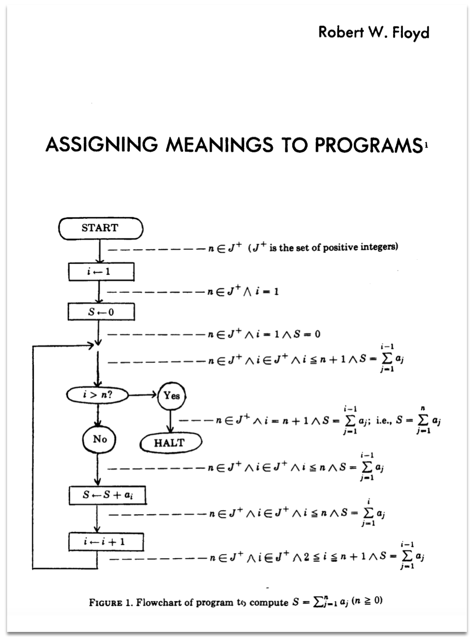
Floyd's paper formulated everything for flow-charts

In 1969 Tony Hoare reformulated those ideas as

which is what we today call axiomatic semantics or Floyd-Hoare (FH) Logic.

Assertions

The central idea in FH logic is the notion of an assertion which is simply property of a State, that is some fact that is true (or not) about a particular program State.

abbrev Assertion := State -> Prop

For example, the state s defined as s0 [x := 10] [ y := 20] satisfies the following assertions

• λ s -> s x < s y
• λ s -> s x + s y = 30

but does not satisfy the assertions

• λ s -> s x = 0
• λ s -> s x > s y

Floyd-Hoare Triples

A Floyd-Hoare triple is a {{ p }} c {{ q }} where

• p is a pre-condition assertion,
• c is a command, and
• q is a post-condition.

Intuitively, the triple {{ p }} c {{ q }} says that

If

• the command c is executed from a state where the precondition p holds and
• the execution of c terminates,

Then

• upon termination, the postcondition q will hold.

We can state the above precisely by defining when a triple is valid

@[simp]
def Valid (p: Assertion) (c: Com) (q: Assertion) :=
  ∀ s t, p s -> (⟨ c, s ⟩ ==> t) -> q t

notation:10 "⊧" " {{" p "}} " c " {{" q "}}" => Valid p c q

Example: Correctness of imp_sum

We can restate the correctness of imp_sum as a FH triple as

{ p } SKIP    { p }


{ q [[ x := a ]] } x <~ a  { q }


{ a > 15  } x <~ a  { x > 15 }

example : ∀ {n},
  ⊧ {{ fun s => s "x" = n }} imp_sum {{ fun t => t "y" = sum n }}
  := by
  simp_all []
  intros n s t xn imp_step
  simp_all [<-xn]
  apply while_sum
  trivial

Floyd-Hoare Logic

The notion of a valid triple is useful in defining a specification of correctness, but we still have to go through the painful and quite tedious proof of while_sum to actually verify the triple.

Proof Rules

The really clever contribution of Floyd and Hoare was to come up with a recipe comprising a system of proof rules that can be automatically applied to do the verification, without ever directly using the big-step semantics!

These rules are compositional meaning that we derive the triple {P} c {Q} by using sub-derivations on the sub-commands of c.

Rule: Skip

For example, we have a rule for the Skip command that says

---------------- [skip]
⊢ {P} SKIP {P}

That is, for any assertion p we can derive that if p holds before the SKIP then it must hold after as well.

Rule: Assign

  ⊢ { y > 0 }    x <~ y   { x > 0 }

  ⊢ { λ s => s y > 0 }    x <~ y   { λ s => (s x > 0) }

    { λ s => q (s [ x := (aval y s) ]) }    x <~ y    { q }

  --------------------------------------- [assign]
  ⊢ { q [[ x := a ]] }    x <~ a    { q }

Rule: Sequence

The rule for sequencing two commands c1; c2 says that

⊢ {p} c1 {tmp} ⊢ {tmp} c2 {q}

⊢ {p} c1; c2 {q}

⊢ {p} c1 {q}      ⊢ {q} c2 {r}
--------------------------------[seq]
⊢ {p} c1; c2 {r}

That is, ⊢ {p} c1; c2 {r} holds if

1. there is some intermediate assertion q
2. that holds after executing c1 from a {p} state, and
3. c2 then takes all q states to r states.

Rule: Assignment

The rule for assignment is quite tricky.

When can we be sure that some assertion q holds after executing x <~ a ?

Lets look at some examples to build up some intuition.

What assertion can you write for ??? in each of the below?

• {???} x <~ 10 { x > 0 }

• {???} x <~ y { x > 0 }

• {???} x <~ a+b { x + a > 0 }

Can you spot some sort of a pattern?

Indeed, if we want q to be true after the assignment x <~ a then

1. The only change made by the assignment is to x

2. So it must be that q is true before the assignment

3. Except with all occurences of x (in q) replaced with a !

----------------------------- [ assign]
{ q [ x := a ] } x <~ a { q }

Example: Swap

Lets see how the rules for assignment and sequence work for our swap example from above.

{{ s y = b /\ s x = a }}

  z <~ var x ;;

{{ s y = b /\ s z = a }}

  x <~ var y ;;

{{ s x = b /\ s z = a }}

  y <~ var z

{{ s x = b /\ s y = a }}

Rule: If-Then-Else

Lets try to work out the rule for establishing a triple ⊢ {p} IF cond THEN c1 ELSE c2 {q}.

Lets think about this triple:

{ TRUE }

  IF 0 < x

    THEN y <~ x

    ELSE y <~ 0 - x

{ 0 <= y }

What must be true before the IF-THEN-ELSE so that we can be sure that 0 <= y after?

How can we know that the above triple holds?

Can you think of the appropriate triples that must hold for c1 and c2 ? How about the rule

⊢ {P} c1 {Q}    ⊢ {P} c2 {Q}
-------------------------------- [If?]
⊢ {P} IF b THEN c1 ELSE c2 {Q}

Is it "sound" (does it prove invalid triples ?)

Is it "complete" (does it prevent proving valid triples?)

How can we fix the rule?

⊢ {???} c1 {Q}    ⊢ { ??? } c2 {Q}
------------------------------------ [If]
⊢ {P} IF b THEN c1 ELSE c2 {Q}

Lets go back to the example

⊢ {true /\ 0 < x} y <~ x { 0 <= y }   ⊢ {true /\ ¬ 0 < x} y <~ 0 - x { 0 <= y }
-------------------------------------------------------------------------------- [If]
⊢ { true } IF (0 < x) THEN y <~ x ELSE y <~ 0 - x) { 0 <= y }

FH rules are too "tight"

Consider this triple: surely it should be valid but we cannot prove it with our rules :-(

{x = 10} SKIP { x > 0}          (ex1)

The skip rule will let us prove that

⊢ {x=10} SKIP {x=10}

and that

⊢ {x > 0} SKIP {x > 0}

but surely we should also be able to prove {x=10} SKIP {x>0}?

Here's another example.

{x = 0} x <~ x + 1 {x = 1}      (ex2)

The Assign rule will let us prove that {x+1 = 1} x <~ x + 1 {x = 1} but not directly that {x=0} x <~ x + 1 {x=1} ... which seems silly!

Can you think about why the above triples ex1 and ex2 hold?

Bonus Rule: Consequence

How can we encode the above intuition as a rule?

We can relax the FH rules with the rule of consequence shown below.

∀ s. P(s) => P'(s)    ⊢ {P'} c {Q'}     ∀ s. Q'(s) => Q(s)
----------------------------------------------------------- [Consequence]
⊢ {P} c {Q}

This rule says that

• if you can establish the triple ⊢ {P'} c {Q'} then

• you can strengthen the precondition meaning, that if ⊢ {P'} c {Q'} holds then you can replace the P' with any assertion P that is stronger than P' i.e. whenever P is true, P' is also true, and

• you can weaken the postcondition meaning, that if ⊢ {P'} c {Q'} holds then you can replace the Q' with any assertion Q that is weaker than Q' i.e. whenever Q' is true, then Q is also true.

So, for example, we can do

--------------------[skip]
⊢ {x=10} SKIP {x=10}              x=10 => x>0
---------------------------------------------[conseq]
⊢ {x=10} SKIP {x>0}


                    ------------------[skip]
x=10 => x>0         ⊢ {x>0} SKIP {x>0}
--------------------------------------------[conseq]
⊢ {x=10} SKIP {x>0}


                   --------------------------[assign]
x=0 => x+1=1       ⊢ {x+1=1} x <~ x + 1 {x=1}
---------------------------------------------[conseq]
⊢ {x=0} x <~ x + 1 {x=1}

Rule: While

Did we forget something: what about WHILE loops?

Lets pick a simple example. How can we prove that after executing the loop below, the value of x is non-negative?

    {{ True }}
    ⊆
    {{ 1000 <= 1000 && 0 <= 0 }}

  i <~ 0;

    {{ 1000 <= 1000 && 0 <= i }}

  x <~ 1000;

    {{ 1000 <= x && 0 <= i }}
  WHILE (i <= n) DO
    {{ 1000 <= x && 0 <= i }}
    ⊆
    {{ 1000 <= x+i && 0 <= i+1 }}

    x <~ x + i;;
    {{ 1000 <= x && 0 <= i+1 }}
    i <~ i + 1
    {{ 1000 <= x && 0 <= i }}
  DONE

{{ 1000 <= x }}

Loop Invariants We need a way to describe an assertion that is true, no matter how many times the loop runs. Such an assertion is called a loop invariant. As the name suggests, the invariant must be true

• base case before the loop starts executing,
• inductive case if the invariant holds before one iteration, it must hold after an iteration.

Lets try to fill in the blanks in the rule below!

⊢ {???} c {???}
-------------------------------- [while]
⊢ {???} WHILE b DO c DONE {???}

When we're done, we should be able to prove (what is the magic I) ?

{true} i <~ 0;; x <~ 0;; WHILE i <= n DO (x <~ x+i;;i<~ i-1) DONE {0<=x}`

Example: sum

{{ x = i /\ 0 <= i }}
=>
{{ 0 + sum x = sum i /\ 0 <= i }}
  y <~ 0
{{ y + sum x = sum i /\ 0 <= i}}

WHILE (0 < x) DO
  {{ y + sum x = sum i /\ 0 <= x }}
  y <~ y + x
  x <~ x - 1

{{ ¬ 0 < x /\ y + sum x = sum i /\ 0 <= x }}
=>
{{ y = sum i}}

Formalizing the Floyd-Hoare Rules

It is pretty straightforward to formalize the FH rules as an inductive predicate in lean.

Formalizing Implication ⊆

First, we need to define implication

open Com

@[simp]
def Implies (p q : Assertion) := ∀ s, p s -> q s

notation:10 p " ⊆ " q => Implies p q

Let us define the assertions tt ("true") and ff ("false") as

@[simp]
def tt : Assertion := fun _ => True

@[simp]
def ff : Assertion := fun _ => False

Now, we can easily prove the following implications, e.g.

theorem p_imp_true  : ∀ {p : Assertion}, p ⊆ tt := by
  simp []

theorem false_imp_p : ∀ {p : Assertion}, ff ⊆ p := by
  simp []

example : (λ s => s x = 10) ⊆ (λ s => s x > 0 ) := by
  intros s x_10
  simp_all []

Formalizing Substitution

Next, lets formalize the idea of "substitution" as appears in the Assign rule.

⊢ { Q[x := a] } x <~ a { Q }

What, exactly, does it mean for Q to hold with the value of x replaced by a ?

notation:10 q "[[ " x ":=" a "]]" => fun s => q (s [ x := (aval a s) ])

Lets go and revisit our examples from above:

NOTE The funext s tactic lets us prove two functions are equal by proving they produce the same (equal) result on all inputs s.

-- 1. `{true} x <~ 10  { 0 < x }`
example : ((λ s => 0 < s x) [[ x := 10 ]]) = tt := by
  funext
  simp [aval, upd]

-- 2. `{0 < y} x <~ y  {0 < x}`
example : ((λ s => 0 < s x) [[ x := var y ]]) = (λ s => 0 < s y) := by
  funext
  simp [aval, upd]

theorem implies_refl : ∀ p, p ⊆ p := by
  intro p s h
  assumption

Formalizing The Proof Rules

inductive FH : Assertion -> Com -> Assertion -> Prop where

  | Skip              : ∀ {p},
                          FH p Skip p

  | Assign            : ∀ {p x a},
                          FH (p [[ x := a ]]) (x <~ a) p

  | Seq               : ∀ {p c1 c2 q r},
                          FH p c1 q -> FH q c2 r ->
                          FH p (c1 ;; c2) r

  | If                : ∀ {p b c1 c2 q},
                        FH (fun s => p s /\   bval b s) c1 q -> FH (fun s => p s /\ ¬ bval b s) c2 q ->
                        FH p (If b c1 c2) q

  | While             : ∀ {p b c},
                        FH (fun s => p s /\ bval b s) c p ->
                        FH p (While b c) (fun s => p s /\ ¬ bval b s)

  | CnsL              : ∀ {p' p c q},
                        FH p c q ->
                        (p' ⊆ p) ->
                        FH p' c q
  | CnsR              : ∀ {p c q q'},
                        FH p c q ->
                        (q ⊆ q') ->
                        FH p c q'

notation:10 "⊢" " {{" p "}} " c " {{" q "}}" => FH p c q

Examples, Mechanized

Swap

Recall the informal proof of swap above

{{ y = b /\ x = a }}    p

  z <~ var x ;;

{{ y = b /\ z = a }}    p0

  x <~ var y ;;

{{ x = b /\ z = a }}    p1

  y <~ var z

{{ x = b /\ y = a }}    q

Lets formally prove the above using the FH rules. (Yuck, still gross!)

theorem swap_correct : ∀ {a b : Val},
  ⊢ {{ λ s => (s y = b /\ s x = a) }}
    swap
    {{ λ s => (s x = b /\ s y = a) }}
  := by
  intros a b
  generalize hp  : (λ (s: State) => (s y = b /\ s x = a)) = p
  generalize hp0 : (λ (s: State) => (s y = b /\ s z = a)) = p0
  generalize hp1 : (λ (s: State) => (s x = b /\ s z = a)) = p1
  generalize hq  : (λ (s: State) => (s x = b /\ s y = a)) = q
  have s0 : ⊢ {{ p }}  z <~ var x {{ p0 }} := by
    simp [<-hp, <-hp0]
    apply FH.CnsL; apply FH.Assign; simp [aval,upd]
  have s1 : ⊢ {{ p0 }} x <~ var y {{ p1 }} := by
    simp [<-hp0, <-hp1]
    apply FH.CnsL; apply FH.Assign; simp [aval,upd]
  have s2 : ⊢ {{ p1 }} y <~ var z {{ q  }} := by
    simp [<-hp1, <-hq]; apply FH.CnsL; apply FH.Assign; simp [aval,upd]
  simp [swap]
  constructor
  assumption
  constructor
  assumption
  assumption

Loop

Recall the informal proof of loop above

{{ True }}

  i <~ 0;

  x <~ 0;

  WHILE (i <= n) DO

    x <~ x + i;;

    i <~ i - 1

  DONE

{{ 0 <= x }}

EXERCISE: Formally prove the above using the FH rules.

Sum

Finally,

{{ x = i /\ 0 <= i }}
=>
{{ 0 + sum x = sum i /\ 0 <= i }}
  y <~ 0
{{ y + sum x = sum i /\ 0 <= i}}

WHILE (0 < x) DO
  {{ y + sum x = sum i /\ 0 <= x }}
  y <~ y + x
  x <~ x - 1

{{ ¬ 0 < x /\ y + sum x = sum i /\ 0 <= x }}
=>
{{ y = sum i}}

def wsum_inv (i:Nat) : Assertion := λ s => s "y" + sum (s "x") = sum i

theorem y0_fh : ⊢ {{λ s => s x = i }} (y <~ 0) {{wsum_inv i }} := by
  generalize h' : (λ (s:State) => s x = i)  = p'
  generalize h  : (wsum_inv i [[ y := 0 ]]) = p
  have aa : p' ⊆ p := by simp_all [<-h', <-h, Implies, wsum_inv, upd, aval]
  have bb : ⊢  {{ p }}  (y <~ 0) {{wsum_inv i }} := by simp [<-h]; apply FH.Assign
  apply FH.CnsL
  assumption
  assumption

theorem csum_fh : ⊢ {{λ s => wsum_inv i s /\ (bval (0 << "x") s)}} csum {{wsum_inv i }} := by
  generalize h1 : (wsum_inv i [[ x := x - 1 ]]) = q1
  generalize h2 : (q1 [[ y := y + x ]])         = q2
  have c1   : ⊢ {{ q1 }} x <~ x - 1 {{wsum_inv i }} := by simp_all [<-h1]; apply FH.Assign
  have c2   : ⊢ {{ q2 }} y <~ y + x {{ q1 }}        := by simp_all [<-h2]; apply FH.Assign
  have c12  : ⊢ {{ q2 }} csum {{wsum_inv i }}       := by apply FH.Seq; assumption; assumption
  have imp1 : (λ s => wsum_inv i s /\ 0 < s x ) ⊆ q2 := by
    simp_all [<-h2, <-h1, upd, Implies, bval, aval, wsum_inv]
    by_cases (x = y) <;> simp_all []
    .case neg =>
      intros s h1 h2
      generalize hx : s x = sx
      cases sx <;> simp_all [sum, Nat.add_assoc]
  apply FH.CnsL
  apply c12
  simp_all [bval, aval]

theorem imp_sum_fh : ⊢ {{ λ s => s "x" = i }} imp_sum {{ λ s => s "y" = sum i }} := by
  have wsum_fh : ⊢ {{wsum_inv i }} wsum {{ λs => wsum_inv i s /\ ¬ (bval (0 << x) s) }} := by
    apply FH.While; apply csum_fh
  have imp_sum' : ⊢ {{ λ s => s "x" = i }} imp_sum {{ λ s => wsum_inv i s /\ ¬ (bval (0 << "x") s)}} := by
    apply FH.Seq; apply y0_fh; apply wsum_fh
  have wsum_exit : (λ s => wsum_inv i s /\ ¬ (bval (0 << "x") s)) ⊆ (λ s => s "y" = sum i) := by
    simp_all [wsum_inv, Implies, bval, aval, sum]; intros; simp_all [sum]
  apply FH.CnsR
  apply imp_sum'
  apply wsum_exit

Soundness of Floyd-Hoare Logic

The great thing about formalizing the definition of Validity and the proof rules is that we can now prove that we did not just make stuff up.

That is, we can prove that the Floyd-Hoare logic is sound meaning that if we can only derive valid triples in the logic. That is, if the proof rules let us conclude the triple ⊢ {{p}} c {{q}} then that triple is in fact valid.

theorem fh_sound :  ( ⊢ {{ p }} c {{ q }} ) -> ( ⊧ {{ p }} c {{ q }} )  := by
  sorry

To recap: the Floyd-Hoare rules give us a sound way to construct proofs of programs, but, lets be honest, the construction is a real PITA.

Next, lets see how to dramatically automate these proofs using verification conditions.

import Cse230wi25.BigStep
import Cse230wi25.L07Axiomatic

set_option pp.fieldNotation false
set_option pp.proofs true

Automating Floyd-Hoare with Verification Conditions

FH rules are nice but still quite tedious to use, because it seems like we need to spell out

1. where to apply which rule
2. how exactly the rules of consequence work

etc.

In fact, the rules are mostly syntax directed meaning that there is exactly one rule that can be applied for each kind of term.

• The rules of consequence
• The loop invariant

Next, lets see how we can automate away more or less everything except the above.

Annotated Commands

Lets assume that the programmer has annotated their code with the loop invariant, so we can define a ACom type which looks just like the previous Com except for the loop constructor which is now of the form While inv b c case, so the inv is baked into the code.

inductive ACom where
  | Skip   : ACom
  | Assign : Vname -> Aexp -> ACom
  | Seq    : ACom  -> ACom -> ACom
  | If     : Bexp  -> ACom -> ACom -> ACom
  | While  : Assertion -> Bexp  -> ACom -> ACom

open ACom

In fact, if we erase the inv from each while, we can convert an ACom program back into the old Com programs.

@[simp]
def erase (c : ACom) : Com :=
  match c with
  | ACom.Skip        => Com.Skip
  | ACom.Assign x a  => Com.Assign x a
  | ACom.Seq c1 c2   => Com.Seq     (erase c1) (erase c2)
  | ACom.If b c1 c2  => Com.If b    (erase c1) (erase c2)
  | ACom.While _ b c => Com.While b (erase c)

As before we can define some "notation" to make it easier to write ACom programs.

|- {λ s => inv s /\ bval b s} c {λs => inv s}

One lean-y way to say that inv is an invariant:

∀ {s, t}, ⟨ c , s ⟩ ==> t -> inv s -> bval b s -> inv t

wp : Com -> Assertion -> Assertion

{λ s => inv s /\ bval b s} ⊆ wp c inv

notation:10 x "<~" e  => ACom.Assign x (ToAexp.toAexp e)
infixr:20 ";;"  => ACom.Seq
notation:10 "IF" b "THEN" c1 "ELSE" c2 => ACom.If b c1 c2
notation:12 "WHILE {-@" inv "@-}" b "DO" c "END" => ACom.While inv (ToBexp.toBexp b) c
notation:20 "[|" c "|]" => erase c
notation:10 "⊢" " {|" p "|}" c "{|" q "|}" => FH p (erase c) q

-- REPEAT c UNTIL b == c ;; WHILE (not c) DO c END

Specifically, note the ⊢ {| p |} c {| q |} triple which means that the triple holds for the erased command c.

Weakest Preconditions

The central idea is reformulate the FH rules into the notion of the weakest precondition wp c q which defines the largest set of starting states from which executing the command c will yield a final state in which the assertion q is guaranteed to hold.

@[simp]
def wp (c: ACom) (q : Assertion) : Assertion :=
  match c with
  | ACom.Skip        => q
  | ACom.Assign x a  => q [[ x := a ]]
  | ACom.Seq c1 c2   => wp c1 (wp c2 q)
  | ACom.If b c1 c2  => (λ s => if bval b s then wp c1 q s else wp c2 q s)
  | ACom.While i _ _ => i

@[simp]
def vc (c : ACom) (q : Assertion) : Prop :=
  match c with
  | ACom.Skip        => True
  | ACom.Assign _ _  => True
  | ACom.Seq c1 c2   => vc c1 (wp c2 q) /\ (vc c2 q)
  | ACom.If _ c1 c2  => vc c1 q /\ vc c2 q
  | ACom.While i b c =>
                        -- ((λ s => i s /\ bval b s) ⊆ (wp c i)) /\
                        (∀ s, i s -> bval b s -> wp c i s) /\
                        (∀ s, i s -> ¬ bval b s -> q s) /\
                        vc c i

theorem vc_sound : vc c q -> (⊢ {| wp c q |} c {| q |})
  := by
  intros vcq
  induction c generalizing q
  . case Skip   => constructor
  . case Assign => constructor
  . case Seq    =>
    rename_i c1 c2 ih1 ih2
    simp [vc] at vcq
    cases vcq
    simp []
    constructor
    apply ih1
    assumption
    apply ih2
    assumption
  . case If     => sorry
  . case While  => sorry

/- ----------------------------------------------------------------------------------------------- -/

@[simp]
def vc' (p: Assertion) (c: ACom) (q: Assertion) : Prop := (p ⊆ wp c q) ∧ (vc c q)

theorem vc'_sound : (vc' p c q) -> (⊢ {| p |} c {| q |}) := by
  intros vcq
  cases vcq
  rename_i vc1 vc2
  apply FH.CnsL
  apply vc_sound; assumption
  apply vc1


/- ----------------------------------------------------------------------------------------------- -/

theorem ex_swap : ∀ {a b},
  ⊢ {| λs => s x = a /\ s y = b |}
      (z <~ x) ;;
      (x <~ y) ;;
      (y <~ z)
    {| λs => s x = b /\ s y = a |}
  := by
  intros a b
  apply vc'_sound
  simp [vc', aval, upd]
  intros; constructor <;> assumption

/- ----------------------------------------------------------------------------------------------- -/

theorem ex1 :
  ⊢ {| tt |}
    x <~ 5
    {| λs => s x = 5 |}
  := by
  apply vc'_sound
  simp_all [aval, upd]

/- ----------------------------------------------------------------------------------------------- -/

theorem ex2 :
  ⊢ {| λs => s x = 10 /\ s y = 1 |}  -- (2) ??
      (x <~ x + y) ;;
      (x <~ x + y)
    {| λs => s x = 12 |}  -- (1) ??
  := by
  apply vc'_sound; simp_all [aval, upd]

-- (1) change POST to λ s => s x = 12 /\ s y = 1
-- (2) change PRE  to λ s => s x = 10 /\ s y = 1

/- ----------------------------------------------------------------------------------------------- -/


theorem ex4 :
  ⊢ {| tt |}
    WHILE {-@ tt @-} true DO
      Skip
    END
    {| ff |}
  := by
  apply vc'_sound
  simp [vc', bval]

/-
vc' tt (while {tt} true skip) ff
==
vc (while {tt} true skip) ff

-- (1) tt /\ true => (wp Skip inv)
-- (2) tt /\ not true => ff

-/
  -- simp_all [aval, bval]

/- ----------------------------------------------------------------------------------------------- -/

-- x=100, 100+0, 100+0+1, 100+0+1+2, 100+0+1+2+3,... 100+0+1+2+3+...+(z-1)

theorem ex_loop :
  ⊢ {| tt |}
      (y <~ 0)   ;;
      (x <~ 100) ;;
      (WHILE {-@ λs => 100 <= s x  @-} y << z DO
         ((x <~ x + y) ;;
          (y <~ y + 1))
      END)
    {| λ s => 100 <= s x |}
  := by
  apply vc'_sound
  simp [bval, aval, upd]
  constructor
  . intros s x_100 _
    calc 100 <= s x       := by assumption
         _   <= s x + s y := by simp []
  . intros; assumption


/-
(x:=n, y:=0)
(x:=n-1, y := 1)
(x:=n-2, y := 2)
(x:=n-3, y := 3)
...
(x:=1,   y := n-1)
(x:=0,   y := n)


(x:=0,   y := n)
-/

theorem bob : ∀ {a b}, 0 < a -> a - 1 + (b + 1) = a + b := by
  intros a b a_pos

  cases a
  . contradiction
  . simp_arith []

theorem ex_drain: ∀ {n: Nat},
  ⊢ {| λ s => s x = n |}
      (y <~ 0)
      ;;
      (WHILE {-@ λ s => s x + s y = n @-} 0 << x DO
         ((x <~ x - 1) ;;
          (y <~ y + 1))
      END)
    {| λ s => s y = n |}
  := by
  intro n
  apply vc'_sound
  simp [bval, aval, upd]
  constructor
  . intros s xy_n x_pos; simp [<-xy_n]; apply bob; assumption
  . intros s xy_n x_0; simp_all[]

/-
x:=n, y:=0
x:=n-1, y:=0 +)
x:=n-2, y:=0 +n + (n-1)
x:=n-3, y:=0 +n + (n-1) +(n-2)
...
x:=0  , y:=0 +n + (n-1) +(n-2)+ ...+ 1


-/


theorem imp_sum' : ∀ {n},
  ⊢ {| λ s => s "x" = n |}
      (y <~ 0) ;;
      (WHILE {-@ λs => s y + sum (s x) = sum n @-} (0 << x) DO
        (y <~ y + x) ;;
        (x <~ x - 1)
       END)
    {| λ s => s "y" = sum n |}
  := by
  intros n
  apply vc'_sound
  simp_all [aval, bval, upd]
  constructor <;> repeat constructor
  . case a.left =>
    intros
    rename_i s a b
    generalize hx : s x = vx
    cases vx <;> simp_all [sum, Nat.add_assoc, Nat.add_comm]

  . case a.right =>
    intros
    rename_i s _ _
    generalize hx : s x = vx
    cases vx <;> simp_all [sum, Nat.add_assoc]

import Cse230wi25.BigStep
import Cse230wi25.L05Evidence

set_option pp.fieldNotation false
set_option pp.proofs true

open Aexp
open Bexp
open Com

Small Step Semantics

The big-step semantics we've seen so far lets us write ⟨ c, s ⟩ ==> t to mean that when c:Com starts executing from s:State it can terminate execution in t:State.

This style of defining what a program means was quite useful in that it let us derive:

1. A way of proving when two families of programs are equivalent
2. A way of proving assertions about particular programs, via Floyd-Hoare logic.

However, the big-step semantics do not give us any visibility into what happens "in the middle", e.g. as the execution marches along from s to t.

Sometimes we care about the intermediate sequence of steps because

1. maybe the program does not terminate and still we want to know that nothing "bad" happens during execution, or

2. we want to reason about some low-level operations (e.g. system calls) that happen during the execution, and not just the start/final states, or

3. we want to reason about concurrent executions where we need to talk about the fine-grained interleaved executions of different threads.

Strategy

So instead of saying ⟨ c, s ⟩ ==> t we want to model executions as a series

c₀ -> c₁ -> c₂ -> c₃ -> ...

where

1. Each cᵢ is a Configuration i.e. a snapshot of the entire system,
2. Each cᵢ -> cⱼ is a SmallStep, and we can
3. Link the individual step to arbitrarily long sequences of SmallSteps.

So our strategy has three parts, we have to define a notion of

(1) Configuration (2) SmallStep (3) SmallSteps

IMP

Can you think about how we might do this in lean for our IMP language

c ::= SKIP | x <~ a | c1 ;; c2 | IF b c1 c2 | WHILE b c

Example

Suppose we have a program like

x <~ 10;; y <~ x + 1 ;; z <~ y + 2

What do you think the sequence of configurations c₀ -> ... might look like?

[ x := 0, y := 0, z := 0 ]

(y <~ 12 ;;
z <~ 1000 ;;
(IF 100 < x THEN y <~ y+10 ELSE z <~ z+20)

y <~ 12

[ x := 0, y := 12, z := 0 ]

z <~ 1000 ;;
(IF 100 < x THEN y <~ y+10 ELSE z <~ z+20)

z <~ 1000

[ x := 0, y := 12, z := 1000 ]

(IF 100 < x THEN y <~ y+10 ELSE z <~ z+20)

[ x := 0, y := 0, z := 0 ]

(y <~ 12 ;; z <~ 1000)
;;
(IF 100 < x THEN y <~ y+10 ELSE z <~ z+20)

"break parens" ~~>

{ (x <~ 10 ;; y <~ x+1) | [x := 0, y:=0] }

~~> assign+semicolon

{ (Skip ;; y <~ x+1) | [x := 10, y:=0] }

~~> skip

{ (y <~ x+1) | [x := 10, y:=0] }

~~> assign

{ Skip | [x := 10, y:=11] }

RULES

--------------------------------------- [skip] { SKIP ;; REST | s } ~~> { REST | s }

{ c | s } ~~> { c' | s' } ------------------------------------------------------------ [semicolon] { (c ;; REST) | s } ~~> { ( c' ;; REST ) | s' }

------------------------------------------------------------ [assign] { (x <~ a ) | s } ~~> { Skip | s [ x := aval a s ] }

bval b s = true --------------------------------------------------- [if-true] { (IF b c1 c2) | s } ~~> { c1 | s}

bval b s = false --------------------------------------------------- [if-true] { (IF b c1 c2) | s } ~~> { c2 | s}

-----------------------------------------------------------[while] { (WHILE b c) | s } ~~> { IF b (c ;; WHILE b c) Skip | s }

An IMP Configuration

To define a small-step semantics the Configuration must have all the information needed to determine the "next" thing that the program does. This means, a configuration should include both

1. the state that maps each Vname to its Value (as in the BigStep semantics), and
2. some representation of the remaining instructions to execute next.

We can model the latter in several ways?

• An "instruction memory" that stores the whole program plus a program counter indicating current instruction?

• Just store the remainder of the program!

We opt for the second option as simpler for IMP: a Configuration is just a pair (or tuple) of the remainder Com and variables' State

abbrev Configuration := (Com × State)

Example

Lets return to our original example:

abbrev com₀ : Com := x <~ 10;; (y <~ x + 1 ;; (z <~ y + 2 ;; Skip))

Suppose we want to execute the program from some starting state st₀ where all the variables are 0

def st₀ : State := λ _ => 0

What are the sequence c₀ -> c₁ -> c₂ -> c₃ of Configuration that we might expect?

def c₀ : Configuration := sorry
def c₁ : Configuration := sorry
def c₂ : Configuration := sorry
def c₃ : Configuration := sorry

One SmallStep

Next, lets try to work out the rules that define the SmallStep relation. As usual, lets use the rules style formulation which says that if the stuff above the line holds, then the stuff below the line holds as well.

Skip

------------------------- [skip]
(Skip;;c, s) -> (c, s)

Assign

----------------------------------------- [assign]
(x <~ a, s) -> (Skip, s [x := aval a s])

Sequence

(c1, s) ~~> (c1', s')
------------------------------- [seq]
(c1;;c2, s) -> (c1';;c2 , s')

If

bval b s = true
------------------------------------ [if-true]
(IF b THEN c1 ELSE c2, s) -> (c1, s)

bval b s = false
------------------------------------ [if-false]
(IF b THEN c1 ELSE c2, s) -> (c2, s)

While

-------------------------------------------------- [while]
(WHILE b DO c, s) -> (IF b (c;;WHILE b c) Skip, s)

Next, lets formulate the above as an inductive SmallStep relation:

((x<~10;; y <~20) ;; z <~ 30) ;; (a <~ 100) | s

~>

((SKIP;; y <~20) ;; z <~ 30) ;; (a <~ 100) | s[x:=10]

~>

(y <~20 ;; z <~ 30) ;; (a <~ 100) | s[x:=10]

~>

(SKIP ;; z <~ 30) ;; (a <~ 100) | s[x:=10][y:=20]

~>

(z <~ 30) ;; (a <~ 100) | s[x:=10][y:=20] ~>

SKIP ;; (a <~ 100) | s[x:=10][y:=20][z:=30]

~>

(a <~ 100) | s[x:=10][y:=20][z:=30]

~>

SKIP | s[x:=10][y:=20][z:=30][a:=100]

inductive SmallStep : Configuration -> Configuration -> Prop where
   | Assign : ∀ {x a s},
                SmallStep (x <~ a, s) (Skip, s [x := aval a s])

   | Seq1   : ∀ {c s},
                SmallStep ((Skip ;; c), s) (c, s)

   | Seq2   : ∀ {c1 c1' c2 s s'},
                SmallStep (c1, s) (c1', s') ->
                SmallStep ((c1 ;; c2) , s) ((c1' ;; c2), s')

   | IfTrue : ∀ {b c1 c2 s},
                bval b s == true ->
                SmallStep (IF b THEN c1 ELSE c2, s) (c1, s)

   | IfFalse : ∀ {b c1 c2 s},
                bval b s == false ->
                SmallStep (IF b THEN c1 ELSE c2, s) (c2, s)

   | While   : ∀ { b c s },
                SmallStep (Com.While b c, s) (Com.If b (c ;; (Com.While b c)) Skip, s)

Many SmallSteps

We can now extend the single SmallStep relation to handle arbitrarily many steps, simply by taking its transitive closure!

That is, recall the definition of star r as taking zero or more r-steps

inductive star {α : Type} (r: α -> α -> Prop) : α -> α -> Prop where
  | refl : ∀ {a : α}, star r a a
  | step : ∀ {x y z : α}, r x y -> star r y z -> star r x z

abbrev Steps := star SmallStep

notation:12 cs "~~>" cs' => SmallStep cs cs'
notation:12 cs "~~>*" cs' => star SmallStep cs cs'

Example: Skip

Lets show that a Skip cannot change the state.

theorem skip_not_change : ∀ {c s t},
  ((Skip, s) ~~>* (c, t)) -> s = t
  := by
  intros c s t skip_steps
  cases skip_steps
  . case refl =>
    trivial
  . case step _ blah _ =>
    contradiction



@[simp]
theorem skip_step : ∀ {s t},
  ((Skip, s) ~~>* (Skip, t)) <-> s=t
  :=
  by
  sorry

Example: Assignments

Lets show that an assignment x <~ a updates the state as follows:

@[simp]
theorem assign_step : ∀ {x a REST s},
  ((((x <~ a) ;; REST), s) ~~>* (REST, s [x := aval a s]))
  :=
  by
  intros
  repeat constructor

Example: A Sequence of Assignments

Lets revisit our old example with (com₀, st₀) ~~>* ...

star_trans: star r x y -> star r y z -> star r x z

example : (com₀, st₀) ~~>* (Skip, st₀[ x := 10 ][ y := 11][ z := 13])
  := by
  apply star_trans; apply assign_step
  apply star_trans; apply assign_step
  apply star_trans; apply assign_step
  simp_all [aval, upd]

SmallStep is Deterministic

Let us prove that the ~~> relation is deterministic, meaning, that each Configuration can only step to at most one other Configuration.

In other words, if a configuration cs ~~> cs1 and cs ~~> cs2 then cs1 and cs2 must be the same.

theorem smallstep_deterministic : ∀ {cs cs1 cs2},
  (cs ~~> cs1) -> (cs ~~> cs2) -> cs1 = cs2
  := by
  intros cs cs1 cs2 step1 step2
  induction step1 generalizing cs2
  . case Assign =>
    cases step2; trivial
  . case Seq1 =>
    cases step2
    trivial
    contradiction
  . case Seq2 c1 c1' c2 s s' step1 ih =>
    cases step2
    contradiction
    rename_i c1'' s'' _
    have foo : (c1', s')= (c1'', s'')  := by
     apply ih; trivial
    simp_all
  . case IfTrue => sorry
  . case IfFalse => sorry
  . case While => sorry

The Equivalence of BigStep and SmallStep Semantics

Next, let us prove that our SmallStep and BigStep definitions are equivalent.

How would we state the above as a theorem?

Helper lemmas about BigStep Semantics

It will be handy to have some @[simp] lemmas to simplify facts about the BigStep semantics. (Lean will automatically apply these everytime we say simp or simp_all.)

theorem BigStep_skip_Iff : ∀ {s t},
  (⟨ Skip, s ⟩ ==> t) <-> (s = t) :=
  by
  intros s t; constructor
  . case mp  => intro h; cases h; simp_all []
  . case mpr => intros; simp_all []; constructor

theorem BigStep_assign_Iff: ∀ {x a s t},
  (⟨ x <~ a, s ⟩ ==> t) <-> (t = (s[x := aval a s]))
  := by
  intros x a s t
  constructor
  . case mp  => intro h; cases h; simp_all []
  . case mpr => intros; simp_all []; constructor

theorem BigStep_seq_Iff: ∀ {c1 c2 s t},
  (⟨ c1 ;; c2, s ⟩ ==> t) <-> (∃ s', (⟨ c1, s ⟩ ==> s') ∧ (⟨ c2, s' ⟩ ==> t)) := by
  intros c1 c2 s t
  apply Iff.intro
  . case mp => intros h; cases h; repeat constructor; repeat assumption
  . case mpr => intros h; cases h; rename_i _ h12; cases h12; constructor; repeat assumption

SmallStep implies BigStep

Next, lets try to prove that if using many small steps we have (c, s) ~~>* (Skip, t) then, in a single big step we have ⟨ c, s ⟩ ==> t.

The only way to do so will be an induction on the sequence of small steps.

theorem smallstep_implies_bigstep' : ∀ {c s t},
  ((c, s) ~~>* (Skip, t)) -> (⟨ c, s ⟩ ==> t)  := by
  intros c s t steps

  generalize h1 : (c, s)    = c_s    at steps --- this is ANF / Nico's tip
  generalize h2 : (Skip, t) = skip_t at steps --- this is ANF / Nico's tip
  induction steps generalizing c s t
  . case refl =>
      cases h1
      cases h2
      constructor

  . case step cs cs1 skip_t step_head step_tail ih =>
      cases h1
      cases h2
      sorry

Yikes! We are stuck! We need some sort of helper lemma that will tell us something about what happens after executing a single small step!

What should that lemma say?

HINT see where we got stuck in the above proof!

theorem step_case : ∀ {c c' s s' t},

  ((c, s) ~~> (c', s')) -> (⟨ c', s' ⟩ ==> t) -> (⟨ c, s ⟩ ==> t)

  := by
  intros c c' s s' t step1 bigstep
  generalize h1 : (c, s)   = cs  at step1 --- this is ANF / Nico's tip
  generalize h2 : (c', s') = cs' at step1 --- this is ANF / Nico's tip
  induction step1 generalizing c c' s s' t <;> cases h1 <;> cases h2
  . case Assign x a s =>
      simp_all [BigStep_assign_Iff, BigStep_skip_Iff]
  . case Seq1 c s =>
      repeat constructor
      assumption
  . case Seq2 c1 c1' c2 s s' _ ih1 =>
      cases bigstep
      rename_i st2 c1'_s'_st2' c2_st2
      constructor
      apply ih1
      apply c1'_s'_st2'
      repeat simp_all []
  . case IfTrue b c1 c2 s hyp =>
      constructor
      simp_all []
      assumption
  . case IfFalse b c1 c2 s hyp =>
      apply BigStep.IfFalse
      simp_all []
      assumption
  . case While b c s =>
      generalize hyp : bval b s = bv
      cases bv
      -- bv = false
      cases bigstep
      repeat simp_all
      apply BigStep.WhileFalse
      assumption
      -- bv = true
      cases bigstep
      simp_all []
      rename_i h_bv h_c_w
      cases h_c_w
      rename_i s' hh
      cases hh
      apply BigStep.WhileTrue
      repeat assumption
      simp_all

We can now use the above lemma to complete the proof of the smallstep_implies_bigstep theorem.

theorem smallstep_implies_bigstep : ∀ {c s t},
  ((c, s) ~~>* (Skip, t)) -> (⟨ c, s ⟩ ==> t)  := by
  intros c s t steps
  generalize h1 : (c, s)    = c_s    at steps --- this is ANF / Nico's tip
  generalize h2 : (Skip, t) = skip_t at steps --- this is ANF / Nico's tip
  induction steps generalizing c s t <;> cases h1 <;> cases h2
  . case refl =>
      constructor
  . case step _ step_head _ ih =>
      apply step_case
      apply step_head
      apply ih
      repeat simp_all []

BigStep implies SmallStep

Next, lets try to prove the other direction that

IF in a single big step we have ⟨ c, s ⟩ ==> t. THEN using many small steps we have (c, s) ~~>* (Skip, t).

<c1, s> ==> s' <c2, s'> ==> t

<c1;;c2 , s > ==> t

Of course, this proof will be by induction on the BigStep derivation.

theorem bigstep_implies_smallstep_stuck : ∀ {c s t},
  (⟨ c, s ⟩ ==> t) -> ((c, s) ~~>* (Skip, t))
  := by
  intros c s t bs
  induction bs
  . case Skip =>
    sorry
  . case Assign s x a =>
    sorry
  . case Seq c1 c2 s1 s2 s3 _ _ sc1 sc2 =>
    sorry
  . case IfTrue =>
    sorry
  . case IfFalse =>
    sorry
  . case WhileFalse b c st b_false =>
    sorry
  . case WhileTrue =>
    sorry

Uh oh, in the Seq case we get stuck because

• we have ⟨ c1, s ⟩ ==> s1, which implies (c1, s) ~~>* (Skip, s1) (by the IH) (c1;; c2, s ) ~~>* (Skip;;c2, s1) ~> (c2,s1) ~~>* (Skip, t)
• we have ⟨ c2, s1 ⟩ ==> t, which implies (c2, s1) ~~>* (Skip, t) (by the IH)

But we need to join the SmallStep sequences for c1 and c2 to get one for c1;;c2.

But how? We need some additional lemma, but what should that lemma say?

theorem seq_steps : ∀ {c1 c1' c2 s s'},
  ((c1, s) ~~>* (c1', s')) ->
  ((c1;;c2, s) ~~>* (c1';;c2, s'))
  :=
  by
  intros c1 c1' c2 s s' steps_c1_c1'
  generalize h1 : (c1, s)   = c1s  at steps_c1_c1'
  generalize h2 : (c1', s') = c1s' at steps_c1_c1'
  induction steps_c1_c1' generalizing c1 c1' c2 s s'
  case refl =>
    rename_i a
    cases h1
    simp_all []
    apply star.refl
  case step  =>
    cases h1
    cases h2
    rename_i c1s'' step_c1_hd _ ih
    apply star.step
    constructor
    apply step_c1_hd
    apply ih
    simp_all []
    simp_all []

We can now use the above lemma to complete the proof...

---------------------------------------------------------------------------------

theorem bigstep_implies_smallstep : ∀ {c s t},
  (⟨ c, s ⟩ ==> t) -> ((c, s) ~~>* (Skip, t))
  := by
  intros c s t bs
  induction bs
  . case Skip =>
    constructor
  . case Assign s x a =>
    apply star.step; constructor; apply star.refl
  . case Seq sc1 sc2 =>
      apply star_trans
      apply seq_steps
      apply sc1
      apply star.step
      apply SmallStep.Seq1
      apply sc2
  . case IfTrue =>
      constructor; apply SmallStep.IfTrue; simp_all []; assumption
  . case IfFalse =>
      constructor; apply SmallStep.IfFalse; simp_all []; assumption
  . case WhileFalse =>
      apply star.step; constructor; apply star_one; constructor; simp_all []
  . case WhileTrue =>
      rename_i c_steps _
      apply star.step; constructor
      apply star.step; constructor
      simp_all []
      apply star_trans
      apply seq_steps c_steps
      apply star.step; constructor
      assumption

----------------------------------------------------------------------------------------------

import Cse230wi25.L05Evidence

set_option pp.fieldNotation false
set_option pp.proofs true

Type Soundness via Small-Step Semantics

Next, lets look at a concrete application of small-step semantics: to prove the correctness of a type checker.

Floating IMP

Our old IMP language has no type-safety issues because, well, every variable is simply a Nat.

Let us extend the set of possible Val to include floating point values as well.

inductive Val where
  | Iv : Int -> Val
  | Fv : Float -> Val
  deriving Repr

open Val

We can have integer values like

#eval (Iv 12)

Or floating point values like

#eval (Fv 3.14)

As before,

• an identifier or variable Vname is just a String and
• a State maps Vname to Val (which is either an Int or a Float).

abbrev Vname := String

abbrev State := Vname -> Val

@[simp] def upd (s: State) (x: Vname) (v: Val) : State :=
  λ y => if y = x then v else s y

notation:10 s " [ " x " := " v " ] " => upd s x v

Arithmetic and Boolean Expressions

Finally, we can extend Aexp to include Int and Float constants, together with the usual binary operations as:

inductive Aexp where
  | Ic  : Int -> Aexp            -- integer constant
  | Fc  : Float -> Aexp          -- floating point constant
  | V   : Vname -> Aexp          -- variable
  | Add : Aexp -> Aexp -> Aexp   -- addition
  deriving Repr

open Aexp

inductive Bexp where
  | Bc   : Bool -> Bexp
  | Not  : Bexp -> Bexp
  | And  : Bexp -> Bexp -> Bexp
  | Less : Aexp -> Aexp -> Bexp
  deriving Repr

open Bexp



class ToAexp (a : Type) where
  toAexp : a -> Aexp


instance : OfNat Aexp (n: Nat) where
  ofNat := Ic n

instance : ToAexp Int where
  toAexp := Ic

instance : ToAexp String where
  toAexp := V

instance : Add Aexp where
  add := fun a1 a2 => Add a1 a2

instance : HAdd String Aexp Aexp where
  hAdd := fun s a => Add (V s) a

instance : HAdd String Int Aexp where
  hAdd := fun s a => Add (V s) (Ic a)

def mkVar (s: String) (i : Nat) : Aexp := V (s!"{s}_{i}")

notation:80 lhs:91 "#" rhs:90 => mkVar lhs rhs

def x := "x"
def y := "y"
def z := "z"

def aexp0 : Aexp := x#1 + y#1 + z#1 + 5

#eval aexp0

Evaluating Expressions

Can you think about why it is a bit tedious (but not impossible!) to define aval for this new Aexp?

So, instead lets define the evaluation of Aexp using an inductive predicate, where we need only define the cases where a value is produced and we can omit the cases where an Int is added to / compared against a Float.

inductive Taval : Aexp -> State -> Val -> Prop where

  | T_Ic  : ∀ {i s},
            Taval (Ic i) s (Iv i)

  | T_Rc  : ∀ {f s},
            Taval (Fc f) s (Fv f)

  | T_V   : ∀ {x s},
            Taval (V x) s (s x)

  | T_AddI : ∀ {a1 a2 s i1 i2},
             Taval a1 s (Iv i1) -> Taval a2 s (Iv i2) ->
             Taval (Add a1 a2) s (Iv (i1 + i2))

  | T_AddF : ∀ {a1 a2 s r1 r2},
             Taval a1 s (Fv r1) -> Taval a2 s (Fv r2) ->
             Taval (Add a1 a2) s (Fv (r1 + r2))

open Taval

inductive Tbval : Bexp -> State -> Bool -> Prop where

  | T_Bc  : ∀ {v s},
            Tbval (Bc v) s v

  | T_Not : ∀ {b v s},
            Tbval b s v ->
            Tbval (Not b) s (!v)

  | T_And : ∀ {b1 b2 v1 v2 s},
            Tbval b1 s v1 -> Tbval b2 s v2 ->
            Tbval (And b1 b2) s (v1 && v2)

  | T_LessI : ∀ {a1 a2 i1 i2 s},
              Taval a1 s (Iv i1) -> Taval a2 s (Iv i2) ->
              Tbval (Less a1 a2) s (i1 < i2)

  | T_LessF : ∀ {a1 a2 r1 r2 s},
              Taval a1 s (Fv r1) -> Taval a2 s (Fv r2) ->
              Tbval (Less a1 a2) s (r1 < r2)

open Tbval


def st0 : State := fun x => match x with
  | "x" => Iv 3
  | "y" => Iv 4
  | _   => Iv 0

Floating Commands

Next, as with plain IMP, we define the type Com of commands, now using the new Aexp and Bexp.

inductive Com where
  | Skip   : Com
  | Assign : Vname -> Aexp -> Com
  | Seq    : Com   -> Com  -> Com
  | If     : Bexp  -> Com  -> Com -> Com
  | While  : Bexp  -> Com  -> Com
  deriving Repr

open Com

infix:10 "<<"  => fun x y => Less x y
infix:10 "<~"  => Com.Assign
infixr:8 ";;" => Com.Seq
notation:10 "IF" b "THEN" c1 "ELSE" c2 => Com.If b c1 c2
notation:12 "WHILE" b "DO" c "END" => Com.While b c

And we can define a SmallStep operational semantics for Com similar to that from the previous lecture.

NOTE Instead of using the functions aval and bval we simply use the relations Taval and Tbval.

abbrev Configuration := (Com × State)


inductive Step : Configuration -> Configuration -> Prop where

   | Assign : ∀ {x a s v},
                Taval a s v ->
                Step (x <~ a, s) (Skip, s [x := v])

   | Seq1   : ∀ {c s},
                Step ((Skip ;; c), s) (c, s)

   | Seq2   : ∀ {c1 c1' c2 s s'},
                Step (c1, s) (c1', s') ->
                Step ((c1 ;; c2) , s) ((c1' ;; c2), s')

   | IfTrue : ∀ {b c1 c2 s},
                Tbval b s true ->
                Step (IF b THEN c1 ELSE c2, s) (c1, s)

   | IfFalse : ∀ {b c1 c2 s},
                Tbval b s false ->
                Step (IF b THEN c1 ELSE c2, s) (c2, s)

   | While   : ∀ { b c s },
                Step (Com.While b c, s) (Com.If b (c ;; (Com.While b c)) Skip, s)

notation:12 cs "~~>" cs' => Step cs cs'

Getting Stuck / Going Wrong

Now that we have Int and Float values, we have introduced the possibility of programs going wrong. For example, we have not defined the meaning of Add (Ic 2) (Fc 3.1) because doing so would require adding an Int and a Float which (suppose we don't have any "casting") is meaningless.

In that case, a program like

x <~ Ic 2 ;;
y <~ Fc 3.1 ;;
z <~ x + y ;;
...

is also meaningless because the addition would get stuck.

How can we make sure that programs are "ok", that is, they do not get stuck?

Type Checking

Well, this is precisely what type checking was invented to solve: to predict -- right when you write your code, that under no circumstances would execution get stuck or go wrong because you mixed up the wrong values for some operation.

Types

For our simple FIMP we require just two types "int" and "float" and so we can model these as a new (lean) type Ty with the constructors (values) TInt and TFloat

inductive Ty where
  | TInt : Ty
  | TFloat : Ty
  deriving Repr

Environments

Next, we need a table or a map that records the Ty for each program variable. Often this structure is called a Type Environment and in PL papers, written using the letter Γ

open Ty

abbrev Env := Vname -> Ty

For example, here is an Environment where every variable is presumed to be an integer.

@[simp] def Γᵢ : Env := fun _ => TInt

Typing Judgments

In Floyd-Hoare logic we proved propositions of the form {p} c {q} that said, roughly, that

IF

• we start execution in a pre-state where p was true and
• execution of c terminates in some post-state

THEN

• the post-state will satisfy the assertion q

Similarly, with type systems we will prove propositions of the form Γ ⊢ e : τ which say that

IF

• the variables in e are assumed to have the types given in Γ

THEN

• the expression e can be determined to have the type τ

We say that e has-type τ in environment Γ.

Typing Rules for Arithmetic Expressions

Next, lets write down some rules that establish this HasType relation, for each of the different kinds of Aexp and Bexp. The rules should let us establish the proposition that Γᵢ ⊢ x + (10 + y) : int i.e. x + (10 + y) has the type int in an environment where all the variables are of type int.

We want the rules to be syntax-directed meaning a single rule should apply for each kind of expression. (Why?)

----------------[int]
Γ ⊢ 3 : ???


----------------[float]
Γ ⊢ 3.14 : ???


----------------[var]
Γ ⊢ x : ???


--------------------[add]
Γ ⊢ a1 + a2 : ???

which we can specify as an inductive predicate:

inductive HasTyA : Env -> Aexp -> Ty -> Prop where

  | Ty_Ic : ∀ {Γ i},
            HasTyA Γ (Ic i) TInt

  | Ty_Fc : ∀ {Γ r},
            HasTyA Γ (Fc r) TFloat

  | Ty_V  : ∀ {Γ x},
            HasTyA Γ (V x) (Γ x)

  | Ty_AddI : ∀ {Γ a1 a2},
              HasTyA Γ a1 TInt -> HasTyA Γ a2 TInt ->
              HasTyA Γ (Add a1 a2) TInt

  | Ty_AddF : ∀ {Γ a1 a2},
              HasTyA Γ a1 TFloat -> HasTyA Γ a2 TFloat ->
              HasTyA Γ (Add a1 a2) TFloat


notation:10 Γ " ⊢ " a " : " τ => HasTyA Γ a τ

Let us check our example

                      -------------[int]    -------------[var]
                      Γᵢ ⊢ 10 : int         Γᵢ ⊢ y : int
------------[var]     -----------------------------------[addI]
Γᵢ ⊢ x : int          Γᵢ ⊢ (10 + y) : int
-----------------------------------------[addI]
Γᵢ ⊢ x + (10 + y) : int

Lets see why having syntax directed rules is useful!

example : Γᵢ ⊢ (V x + (Ic 10 + V y)) : TInt := by
  sorry

Typing Rules for Boolean Expressions

Next, lets work out the rules for Bexp -- here we can just write Γ ⊢ b (and leave out : bool because?)

???
---------------
Γ ⊢ true : ???


???
---------------[not]
Γ ⊢ ¬ b : ???


???
-------------------[and]
Γ ⊢ b1 /\ b2 : ???

???
--------------------[less]
Γ ⊢ a1 < a2 : ???

Lets formalize the above as an inductive predicate:

inductive HasTyB : Env -> Bexp -> Prop where
  | Ty_Bc   : ∀ {Γ v},
              HasTyB Γ (Bc v)

  | Ty_Not  : ∀ {Γ b},
              HasTyB Γ b ->
              HasTyB Γ (Not b)

  | Ty_And  : ∀ {Γ b1 b2},
              HasTyB Γ b1 -> HasTyB Γ b2 ->
              HasTyB Γ (And b1 b2)

  | Ty_Less : ∀ {Γ a1 a2 t} ,
              HasTyA  Γ a1 t -> HasTyA Γ a2 t ->
              HasTyB Γ (Less a1 a2)

notation:10 Γ " ⊢ " a  => HasTyB Γ a

Again, the syntax-directed nature of the rules makes establishing the "has-type" facts super easy!

example : Γᵢ ⊢ (V x + (Ic 10 + V y)) << Ic 29 := by
  sorry

Typing Rules for Commands

Finally, lets work out the rules for typing commands.

What does the typing judgment for a command look like?

QUIZ

Should the following hold?

(1)

Γᵢ ⊢ x <~ 10 ;; Skip ;; y <~ 10 ;; z <~ x + y

(2)

Γᵢ ⊢ x <~ 10 ;; Skip ;; y <~ 1.0 ;; z <~ x + y

What should the rules look like so that we can establish / reject appropriately?

???
---------------[skip]
Γ ⊢ skip


???
---------------[assign]
Γ ⊢ x <~ a


???
-------------------[seq]
Γ ⊢ c1 ;; c2

???
-------------------------[if]
Γ ⊢ if b then c1 else c2

???
-------------------------[while]
Γ ⊢ while b do c

Lets define the above as an inductive predicate

inductive HasTyC : Env -> Com -> Prop where
  | Ty_Skip   : ∀ {Γ},
                HasTyC Γ Skip

  | Ty_Assign : ∀ {Γ x a},
                HasTyA Γ a (Γ x) ->
                HasTyC Γ (x <~ a)

  | Ty_Seq    : ∀ {Γ c1 c2},
                HasTyC  Γ c1 -> HasTyC Γ c2 ->
                HasTyC Γ (c1 ;; c2)

  | Ty_If     : ∀ {Γ b c1 c2},
                HasTyB Γ b -> HasTyC Γ c1 -> HasTyC Γ c2 ->
                HasTyC Γ (IF b THEN c1 ELSE c2)

  | Ty_While  : ∀ {Γ b c},
                HasTyB Γ b -> HasTyC Γ c  ->
                HasTyC Γ (WHILE b DO c END)

notation:10 Γ " ⊢ " c  => HasTyC Γ c

-- Yay for syntax directed!
example : Γᵢ ⊢ "x" <~ Ic 3 ;; "y" <~ (V "x") + (Ic 4) := by
  repeat constructor

Type Soundness

Ok great, so we made up a system of "type checking" rules.

But how do we know the rules are sensible or meaningful ?

How do we know the rules actually tell us something about the programs execution?

That is, right now we have defined two semantics for FIMP:

• Dynamic Semantics i.e. how the programs run via the SmallStep operational semantics; and

• Static Semantics i.e. how the programs type-check via the HasTy rules.

How can we relate or connect these two descriptions of program behavior?

Ultimately, we want to prove that

• If the program was well-typed (statically)
• Then the program will not go bad (dynamically).

But how can we state this property precisely as a theorem?

Preservation If the program does something THEN that thing is expected or predicted

Progress The program does something.

Let's try to formalize this in Lean,

1. for arith expressions,
2. for bool expressions and then,
3. for commands.

Types and their Values

First, let us write down the relationship between each value and its corresponding type.

@[simp] def type(v: Val) : Ty := match v with
  | Iv _ => TInt
  | Fv _ => TFloat

A State s is well-formed with respect to a type environment Γ if every variable's value in s is that specified in Γ

@[simp] def Wf (Γ: Env) (s: State) : Prop :=
  ∀ x, Γ x = type (s x)

notation:10 Γ " ⊧ " s  => Wf Γ s

Arithmetic

Lets start with specifying the preservation and progress properties for Aexp

Preservation

If the program does something THEN that thing is expected or predicted

If the AExp does __________________________ THEN ____________________________

∀ { a } ,

  __________________________________________ ->

  __________________________________________

Progress The program does something.

∀ { a } ,

  __________________________________________ ->

  __________________________________________

Preservation

Now, lets try to prove it!

theorem arith_preservation : ∀ { Γ a τ s v },
  (Γ ⊧ s) -> (Γ ⊢ a : τ) -> Taval a s v -> type v = τ
  := by
  intros Γ a τ s v G_s G_a_t a_s_v
  induction G_a_t generalizing v
  . case Ty_Ic i => cases a_s_v; simp_all
  . case Ty_Fc f => cases a_s_v; simp_all
  . case Ty_V x  => cases a_s_v; simp_all
  . case Ty_AddI a1 a2 _ _ ih1 _ =>
    cases a_s_v
    . simp_all
    . rename_i _ _ av1 _; apply (ih1 av1)
  . case Ty_AddF a1 a2 _ _ ih1 _ =>
    cases a_s_v
    . rename_i _ _ av1 _; apply (ih1 av1)
    . simp_all

Progress

Now, lets try to prove it!

theorem arith_progress': ∀ { Γ a τ s },
  (Γ ⊧ s) -> (Γ ⊢ a : τ) ->  ∃ v, Taval a s v  := by
  intros Γ a τ s G_s G_a_t
  induction G_a_t
  . case Ty_Ic i => repeat constructor
  . case Ty_Fc f => repeat constructor
  . case Ty_V x  => repeat constructor
  . case Ty_AddI => sorry
  . case Ty_AddF => sorry

The (slightly) tricky bit is to prove the progress for a1 + a2 expressions. Lets try to figure out what a helper lemma would look like!

@[simp] def ty_val (t:Ty) (v:Val) : Prop :=
  match t with
  | TInt => ∃ n, v = Iv n
  | TFloat => ∃ n, v = Fv n

theorem arith_preservation_val : ∀ { Γ s a τ v },
  (Γ ⊧ s) -> (Γ ⊢ a : τ) -> Taval a s v -> ty_val τ v
  := by
  intros Γ s a τ v _ _ _
  have hv : type v = τ := by apply arith_preservation; repeat assumption
  cases v <;> simp_all [<-hv]

theorem add_progress: ∀ {Γ a1 a2 τ s},
  (Γ ⊧ s) -> (Γ ⊢ a1 : τ) -> (Γ ⊢ a2 : τ) ->
  (∃ v1, Taval a1 s v1) -> (∃ v2, Taval a2 s v2) ->
  ∃ v, Taval (a1 + a2) s v
  := by
  intros Γ a1 a2 τ s gs gt1 gt2 av1 av2
  cases av1; cases av2; rename_i v1 _ v2 _
  have h1' : ty_val τ v1 := by
    apply arith_preservation_val
    assumption; apply gt1; assumption
  have h2' : ty_val τ v2 := by
    apply arith_preservation_val
    assumption; apply gt2; assumption
  cases τ
  . case TInt   => cases h1'; cases h2'; simp_all; constructor; apply T_AddI; repeat assumption
  . case TFloat => cases h1'; cases h2'; simp_all; constructor; apply T_AddF; repeat assumption

Now we can use add_progress to complete the proof of arith_progress.

theorem arith_progress: ∀ { Γ a τ s },
  (Γ ⊧ s) -> (Γ ⊢ a : τ) ->  ∃ v, Taval a s v  := by
  intros Γ a τ s G_s G_a_t
  induction G_a_t
  . case Ty_Ic i => repeat constructor
  . case Ty_Fc f => repeat constructor
  . case Ty_V x  => repeat constructor
  . case Ty_AddI => apply add_progress; repeat assumption
  . case Ty_AddF => apply add_progress; repeat assumption

Boolean Expressions

These more or less follow the same structure as the arithmetic expressions, except that instead a1 < a2 requires a bit of elbow grease, similar to add_progress.

QUESTION Why don't we need a bool_preservation theorem???

theorem less_progress : ∀ {Γ a1 a2 s v1 v2 τ},
  (Γ ⊧ s) -> (Γ ⊢ a1 : τ) -> (Γ ⊢ a2 : τ) ->
  (Taval a1 s v1) -> (Taval a2 s v2) ->
  ∃ v, Tbval (a1 << a2) s v
  := by
  intros Γ a1 a2 s v1 v2 τ gs gt1 gt2 av1 av2
  have h1' : ty_val τ v1 := by
    apply arith_preservation_val
    assumption; apply gt1; assumption
  have h2' : ty_val τ v2 := by
    apply arith_preservation_val
    assumption; apply gt2; assumption
  cases τ
  . case TInt   => cases h1'; cases h2'; simp_all; constructor; apply T_LessI; repeat assumption
  . case TFloat => cases h1'; cases h2'; simp_all; constructor; apply T_LessF; repeat assumption

theorem bool_progress: ∀ { Γ s } { b : Bexp },
  (Γ ⊧ s) -> (Γ ⊢ b) -> ∃ v, (Tbval b s v)
  := by
  intros Γ s b Gs Gb
  induction Gb
  . case Ty_Bc v =>
    repeat constructor
  . case Ty_Not b' gb' ih =>
    cases ih
    repeat constructor
    assumption
  . case Ty_And b1 b2 Gb1 Gb2 ih1 ih2 =>
    cases ih1; cases ih2
    repeat constructor
    repeat assumption
  . case Ty_Less a1 a2 τ Ga1 Ga2 =>
    have h1 : ∃ v1, Taval a1 s v1 := by apply arith_progress; repeat assumption
    have h2 : ∃ v2, Taval a2 s v2 := by apply arith_progress; repeat assumption
    cases h1; cases h2; apply less_progress; repeat assumption

Commands

What should "preservation" and "progress" theorems look like for Com ?

Preservation

If the program does something THEN that thing is expected or predicted

If the Com does __________________________ THEN ____________________________

∀ { c } ,

  __________________________________________ ->

  __________________________________________

Progress The program does something.

∀ { c } ,

  __________________________________________ ->

  __________________________________________

Commands: Preservation

Let us split the preservation into two separate theorems the Com and State parts of the Configuration. Preservation follows directly by manipulating the typing rules.

theorem preservation1_com : ∀ { Γ } { c c' : Com } { s s' : State },
  (Γ ⊧ s) -> (Γ ⊢ c) -> ((c, s) ~~> (c', s')) -> (Γ ⊢ c')
  := by
  intros Γ c c' s s' wf_s ty_c step
  induction ty_c generalizing c' s s' <;> cases step <;> repeat trivial
  . case Ty_Assign.Assign => constructor
  . case Ty_Seq.Seq2      => rename_i ih _ _ _; constructor; apply ih; repeat trivial
  . case Ty_While         => repeat (constructor <;> repeat trivial)

theorem update_ty : ∀ { Γ s x v },  (Γ ⊧ s) -> (type v = Γ x) -> (Γ ⊧ s [x := v]) := by
  intros Γ s x v v_ty_x wf_s y
  by_cases (y = x) <;> simp_all

theorem preservation1_state : ∀ { Γ } { c c' : Com } { s s' },
  (Γ ⊢ c) -> (Γ ⊧ s) -> ((c, s) ~~> (c', s')) -> (Γ ⊧ s')
  := by
  intros Γ c c' s s' ty_c wf_s step_c_c'
  induction ty_c generalizing c' s <;> cases step_c_c' <;> repeat trivial
  . case Ty_Assign.Assign => apply update_ty; trivial; apply arith_preservation; repeat trivial
  . case Ty_Seq.Seq2      => rename_i ih1 _ _ _; apply ih1; repeat trivial

Commands: Progress

Progress requires using the arith_progress and bool_progress.

theorem progress1 : ∀ { Γ s } { c : Com},
  (Γ ⊧ s) -> (Γ ⊢ c) ->  ¬ (c = Skip) -> ∃ c' s', (c, s) ~~> (c', s')
  := by
  intros Γ s c wf_s ty_c not_skip
  induction ty_c <;> repeat trivial
  . case Ty_Assign x a a_ty =>
    cases (arith_progress wf_s a_ty)
    repeat constructor
    repeat assumption
  . case Ty_Seq    =>
    rename_i c1 c2 c1_ty c2_ty ih1 ih2
    by_cases (c1 = Skip)
    . case pos =>
      apply Exists.intro; apply Exists.intro
      simp_all
      apply Step.Seq1
    . case neg c1_notskip =>
      cases (ih1 c1_notskip)
      rename_i c1' step1'
      cases step1'
      apply Exists.intro; apply Exists.intro;
      apply Step.Seq2
      repeat trivial
  . case Ty_If     =>
    rename_i b c1 c2 b_ty _ _ _ _
    cases (bool_progress wf_s b_ty)
    rename_i bv hbv
    cases bv
    . case intro.false =>
      apply Exists.intro; apply Exists.intro;
      apply Step.IfFalse; assumption
    . case intro.true =>
      apply Exists.intro; apply Exists.intro;
      apply Step.IfTrue; assumption
  . case Ty_While =>
    apply Exists.intro; apply Exists.intro;
    apply Step.While

Commands: Multiple Steps!

We would like to say something not just about a single step but about all the configurations that may be reached by zero or more steps.

abbrev Steps := star Step

notation:12 cs "~~>*" cs' => Steps cs cs'

Lets try to work out what preservation and progress look like for many steps.

Preservation

If the program does something THEN that thing is expected or predicted

∀ { c } ,

  __________________________________________ ->

  __________________________________________

Progress The program does something.

∀ { c } ,

  __________________________________________ ->

  __________________________________________

theorem progress : ∀ { Γ } { c c' : Com } { s s' : State},
  (Γ ⊧ s) -> (Γ ⊢ c) -> ((c, s) ~~>* (c', s')) -> ¬ (c' = Skip) ->
  ∃ c'' s'', (c', s') ~~> (c'', s'')
  := by
  intros Γ c c' s s' wf_s ty_c steps not_skip
  generalize h : (c, s)   = cs at steps --- this is ANF / Nico's tip
  generalize h : (c', s') = cs' at steps --- this is ANF / Nico's tip
  induction steps generalizing Γ c s c' s'
  . case refl =>
    rename_i h1
    cases h1
    cases h
    apply (progress1 wf_s ty_c not_skip)
  . case step =>
    rename_i cs1 cs2 cs3 step1 step_rest ih hh
    cases cs2
    rename_i c2 s2
    cases h
    cases hh
    have ty_c2 : HasTyC Γ c2 := by apply (preservation1_com wf_s ty_c step1)
    have wf_s2 : Wf Γ s2     := by apply (preservation1_state ty_c wf_s step1)
    apply (ih wf_s2 ty_c2 not_skip)
    repeat trivial